Functional biology has played an increasingly important role in elucidating and understanding ecological differences among organisms (Webb, 1982, 1984; Denny, 1988; Norberg, 1990; Niklas, 1992; Wainwright and Reilly, 1994; Vogel, 1994). Many ecologically relevant functional analyses require the estimation of first and second derivatives using numerical differentiation. For example, some measures of functional performance (e.g. maximum velocity, acceleration and turning curvature) for behaviors important to fitness (e.g. feeding strikes, escape responses, maneuvering) are estimated using first and second derivatives of a discretely sampled function. Additionally, accurate estimates of the entire history of velocity, acceleration and turning curvature, over some
discrete amount of time, are critical for investigating biomechanical models of animal movements that occur during feeding and locomotion. Robust biomechanical models of animal motion can lead to predictions of performance and, ultimately, ecological variation.
Numerical differentiation necessarily suffers from the magnification of small errors introduced during the digitizing process. Smoothing and filtering are two distinct, but related, classes of methods for estimating and removing this error. These two classes reflect different ‘ways of seeing’ measurement error. In smoothing, the estimated error is removed by fitting a function that follows the central trend of the data and replacing the observed values with the expected JEB1331
Functional biologists employ numerical differentiation for many purposes, including (1) estimation of maximum velocities and accelerations as measures of behavioral performance, (2) estimation of velocity and acceleration histories for biomechanical modeling, and (3) estimation of curvature, either of a structure during movement or of the path of movement itself. I used a computer simulation experiment to explore the efficacy of ten numerical differentiation algorithms to reconstruct velocities and accelerations accurately from displacement data. These algorithms include the quadratic moving regression (MR), two variants of an automated Butterworth filter (BF1–2), four variants of a method based on the signal’s power spectrum (PSA1–4), an approximation to the Wiener filter due to Kosarev and Pantos (KPF), and both a generalized cross-validatory (GCV) and predicted mean square error (MSE) quintic spline. The displacement data simulated the highly aperiodic escape responses of a rainbow trout Oncorhynchus mykiss and a Northern pike Esox lucius (published previously). I simulated the effects of video speed (60, 125, 250, 500 Hz) and magnification (0.25, 0.5, 1 and 2 screen widths per body length) on algorithmic performance. Four performance measures were compared: the per cent error of the estimated maximum velocity
(Vmax) and acceleration (Amax) and the per cent root mean square error over the middle 80 % of the velocity (VRMSE) and acceleration (ARMSE) profiles.
The results present a much more optimistic role for numerical differentiation than suggested previously. Overall, the two quintic spline algorithms performed best, although the rank order of the methods varied with video speed and magnification. The MSE quintic spline was extremely stable across the entire parameter space and can be generally recommended. When the MSE spline was outperformed by another algorithm, both the difference between the estimates and the errors from true values were very small. At high video speeds and low video magnification, the GCV quintic spline proved unstable. KPF and PSA2–4 performed well only at high video speeds. MR and BF1–2 methods, popular in animal locomotion studies, performed well when estimating velocities but poorly when estimating accelerations. Finally, the high variance of the estimates for some methods should be considered when choosing an algorithm.
Key words: locomotion, velocity, acceleration, performance, biomechanics, movement analysis, fast start, Fourier analysis, spline analysis, filters, simulated data.
Summary
Introduction
ESTIMATING VELOCITIES AND ACCELERATIONS OF ANIMAL LOCOMOTION: A
SIMULATION EXPERIMENT COMPARING NUMERICAL DIFFERENTIATION
ALGORITHMS
JEFFREY A. WALKER*
Department of Zoology, Field Museum, Roosevelt Road at Lake Shore Drive, Chicago, IL 60605, USA *e-mail: [email protected]
or ‘smoothed’ values. This method is probably most intuitive to biologists who are familiar with errors around trend lines in many other biological problems. In filtering, the trend, or signal, is modeled as a high-amplitude, low-frequency component of the data, and the error, or noise, is removed by filtering out the low-amplitude, high-frequency components from the signal. Filtering is probably most intuitive to engineers who are familiar with noisy signals in many different systems.
Numerous smoothing and filtering algorithms are available, but few objective reasons have been offered to choose one algorithm over another. This lack of guidance is unfortunate because, while most of these algorithms produce similar first and second derivatives for data with trivial levels of digitizing error, they produce widely divergent derivative estimates for large and more realistic levels of error. Many biologists investigating (nonhuman) animal movement have shown little concern for the accuracy of the numerical differentiation algorithms employed (but see Rayner and Aldridge, 1985; Harper and Blake, 1989). By contrast, numerical differentiation algorithms have been intensively developed and evaluated in the human movement sciences (Hatze, 1981; Wood, 1982; Woltring, 1985, 1986a; D’Amico and Ferrigno, 1992; Corradini et al. 1993; Gazzani, 1994; Giakas and Baltzopoulos, 1997a). Unfortunately, the performance of numerical differentiators in the human movement sciences has been limited to data sampled at relatively low frequencies (50–100 Hz). Because accuracy in numerical differentiation varies with sampling frequency (Harper and Blake, 1989), animal biologists using high-speed video should exercise caution when extrapolating results from human movement studies.
In this study, a computer simulation experiment is used to compare the performance of ten numerical differentiation algorithms and to explore the effects of video magnification and video speed on algorithmic performance. Algorithmic performances were evaluated by comparing estimated velocities and accelerations with reference values from a function known a priori. I focused on two aspects of algorithmic performance: (1) the accuracy of an algorithm’s reconstruction of velocities and accelerations throughout the duration of a movement (which may be arbitrarily defined) and (2) the accuracy of estimated maximum velocities and accelerations.
Materials and methods
Generation of simulated data
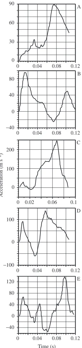
To create reference velocity and acceleration histories with known values, I digitized the acceleration profiles illustrated in Figs 3–7 of Harper and Blake (1990). These data were from two escape responses of a rainbow trout Oncorhynchus mykiss and three escape responses of a Northern pike Esox lucius and were originally measured with an accelerometer surgically implanted into the body of the individual (Harper and Blake, 1990). The figures were digitized with between 93 and 132
unequally spaced points. For each raw trace, I used a linear regression between each pair of adjacent points as an interpolator and divided the measured function into 8001 equally spaced points. At a sampling rate of 60 Hz, 5–6 points would be sampled from the reference data, which is below the minimum number of points for some of the algorithms. I therefore added enough points with zero acceleration to the beginning of the reference sequences to allow an additional two points when sampled at 60 Hz. Because the same reference sequences were used for all simulations, this addition increased the number of points sampled at 125, 250 and 500 Hz by 4, 8 and 16, respectively. The total numbers of points, Nref, in the
reference profiles for Figs 3–7 of Harper and Blake (1990) were 10 199, 10 024, 10 527, 10 199 and 10 077, respectively. The reference figures are illustrated in Fig. 1. I generated the five reference displacement profiles by doubly integrating the acceleration data using:
and
where ∆t is the time between points in the reference sequence, aiis the reference acceleration, viis the reference velocity and
yiis the reference displacement at time i. The initial velocity and acceleration were set to zero.
Four different levels (60, 125, 250 and 500 Hz) of video speed (VS) were simulated by sampling every kth point of the
Nrefreference points where:
The period, T, of each reference response was estimated from Figs 3–7 of Harper and Blake (1990). I simulated the random effect of starting the camera anywhere within the half-interval 1/(2VS) by initiating sampling at a random time, r, within the range 0⭐r⭐1/(2VS). I simulated the effect of digitizing pixels, which have discrete values, rather than actual displacements, with continuous values, by transforming the sampled distances into pixels:
where BL is the body length of the fish, HR is horizontal resolution and VM (video magnification) is the number of screen widths contained in one fish body length. I used the fork length of each individual (Harper and Blake, 1990) for BL and a typical horizontal resolution of a high-speed video camera (480 lines) for HR. Measurement error is a function of both the magnitude and frequency of incorrectly digitizing the correct pixel and the amount of magnification (level of VM). I simulated measurement error by varying VM and holding the
y* = round yi iHR×VM
BL , (4)
(
)
k = Nref−1
VS × T . (3)
yi=∆t vi+ vi–1
2 + yi–1 (2)
(
)
,vi=∆t
ai+ ai –1
2 + vi–1 (1)
magnitude and frequency of incorrectly digitized pixels constant. Four different levels of VM were simulated: 0.25×, 0.5×, 1×and 2×, where ×represents screen widths per body length (hence, 0.5 of the body length would be visible within the screen width at 2×). I added a one pixel error to N/3 points, where N is the number of sampled points in the simulated sequence. In a test of digitizing error using a clearly defined marker on a moving fish, five-sixths of the trials had the same pixel value while one-sixth differed by one pixel; hence, my simulated error is large, by comparison. The sign of the added error was random. Finally, error was constrained to occur at the points in which the fish was moving (i.e. no error was added to points sampled from the initial sequence of zero displacement).
The level of error, or roughness of the data, can be compared with other data sets using:
(Corradini et al. 1993). Corradini et al. (1993) noted that ‘Lanshammar (1982a) considered a value of 0.87 to be realistic whereas Hatze (1981) judged data with [r] equal to 7.28 to be severely contaminated by noise’. The mean values of r for VM of 2×, 1×, 0.5× and 0.25× were 0.57, 1.14, 2.25 and 4.4, respectively.
To generate a sample of estimates within each VM×VS combination, I sampled the reference sequence 100 times, each time starting the sampling from a random time and adding one pixel error of random sign to one-third of the sampled values. With each simulated sequence, I estimated instantaneous velocities and accelerations using the methods described below and converted these estimates back into the original units (m s−2) using the inverse of equation 4.
Four performance statistics were compared among the algorithms. VRMSE is the per cent root mean square error
(RMSE) of the velocity estimates, vˆi, taken with respect to the
true velocities, v, for the middle 80 % of the sampled times within the sequence:
The first and last 10 % of the data points were excluded from the computation of RMSE to avoid the large edge effects that occur with some of the algorithms. Vmax is the per cent error
of the estimated maximum velocity:
ARMSE , the per cent root mean square error of the acceleration
estimates, and Amax, the per cent error of the estimated
Vmax=
max(vi) – max(vi)
max(vi)
×100 . (7)
VRMSE=
(vi– vi)
Σ
i = round(0.1 N) round(0.9N)
(vi)
Σ
i = round(0.1N)
round(0.9N) ×100 . (6)
r = σσsignalnoise ×100 (5)
Time (s)
A
0 30 60 90
0 0.04 0.08 0.12
−40 0 40 80
0 0.04 0.08 0.12 B
100 200
0
0 0.02 0.06 0.1 C
Acceleration (m s
−
2)
−100 100
0
0 0.04 0.08 0.12 D
−40 0 40 80 120
0 0.04 0.08 0.12 E
[image:3.609.99.239.72.664.2]maximum acceleration, were calculated by substituting accelerations for velocities in equations 6–7.
Numerical differentiation algorithms compared (Table 1) Moving regression (MR)
Given a vector of N sampled positions, yi, measured every
∆t seconds, derivatives are commonly estimated by backwards, forwards or first central differences:
and
respectively. While these simple estimates using linear regression are extremely sensitive to measurement error, polynomial regressions through five or more points are potentially more robust (Lanshammar, 1982a). Lanczos (1956) described a simple solution to smooth noisy data and estimate first and second derivatives based on a five-point piecewise quadratic polynomial regression. In the method of Lanczos (1956), derivatives are not computed by differentiating a quadratic function but, instead, are estimated directly by taking a weighted average of the two (first derivative) or four (second derivative) smoothed values immediately prior to and following the point of interest. I implemented the MR algorithm directly from Lanczos (1956) with no modification. Prior to the numerical differentiation, I used the fourth-order central differences to smooth the raw data (Lanczos, 1956).
Automated bidirectional second-order Butterworth digital filter (BF)
I used the bidirectional second-order Butterworth filter described in Winter (1990), but employed a fully automated method for choosing the optimal cut-off frequency, fc. Winter
(1990) developed a semi-automatic method to find fcfrom the
regression of root mean square error (RMSE), measured across a range of cut-off frequencies, against these cut-off frequencies. In this residual analysis (RA), the RMSE is the error from the unfiltered function, not the true function, which is unknown. A problem with implementing this as a generalized ‘black-box’ procedure is that it is unclear which frequencies to include in the linear regression.
Instead of using Winter’s (1990) approach, I employed an autocorrelation analysis of the residuals and used two different criteria for finding the optimal cut-off frequency. For each potential cut-off frequency between 0 and 0.5fs
(where fs is the sampling frequency), taken at 0.1 Hz
intervals, I computed the autocorrelation function of the N residuals. The sum of the squared autocorrelations (SSRA) at each lag, normalized by the autocorrelation at lag zero, was used as a measure of the residual autocorrelation. The first optimal fcwas chosen as the value resulting in the minimum
SSRA (Cappello et al. 1996).
For the second estimate of the optimal fc, I compared the
observed SSRA at each potential fc with the upper ninetieth
percentile of SSRAs computed from N random normal variates. Any set of residuals with an observed SSRA below this ninetieth percentile is considered not significantly different from a random time series. The optimal fcwas chosen as the
lowest value that resulted in a ‘random’ SSRA. I refer to the minimization method as BF1 and the comparison with a random time series method as BF2.
For both variants of the optimal Butterworth filter, I first extrapolated the data using a quadratic polynomial. At each tail of the series, I used a quadratic polynomial through seven (if N⭓10) or five (if N<10) points and added N/2 points at equal intervals using the quadratic coefficients. This point extrapolation has been shown to improve the efficacy of a filtered function and its derivatives (D’Amico and Ferrigno, 1990; Smith, 1989). Smith (1989) found that a linear extrapolation method was the best of several alternatives (but not including a quadratic polynomial method). In my exploration of several extrapolation algorithms, I found a quadratic polynomial extrapolation performed better than a linear extrapolation.
dy d t =
1
2∆t
(
yi– yi–1) (
+ yi+1– yi)
, (10)dy d t =
1
∆t(yi+1– yi) (9)
dy d t =
1
∆t(yi– yi–1), (8)
Table 1. Summary information on the ten algorithms compared in this study
MR Five-point quadratic moving regression (Lanczos, 1956)
BF1 Butterworth filter using minimized autocorrelation optimization (Winter, 1990; Cappello et al. 1996)
BF2 Butterworth filter using random residual optimization (Winter, 1990; this study)
PSA1 Power spectrum analysis using SF=1 (D’Amico and Ferrigno, 1990, 1992)
PSA2 Power spectrum analysis using SF=2 (D’Amico and Ferrigno, 1990, 1992)
PSA3 Power spectrum analysis using Butterworth filter (D’Amico and Ferrigno, 1990, 1992; this study)
PSA4 Power spectrum analysis using quintic spline filter (D’Amico and Ferrigno, 1990, 1992; this study)
KPF Kosarev–Pantos approximation of the Wiener filter (Gazzani, 1994)
GCV Generalized cross-validatory quintic spline (Woltring, 1985, 1986a)
MSE Predicted mean square error quintic spline (Woltring, 1985, 1986a)
Power spectrum analysis (PSA)
D’Amico and Ferrigno (1990) developed a method of finding the optimal fcfrom the power spectrum density of the
observed data. D’Amico and Ferrigno (1992) referred to this method as the linear-phase autoregressive model-based derivative assessment algorithm (LAMBDA). They discussed a parameter, the sharpening factor (SF), that increases or decreases the length of the filter window used in the filter. A decrease in SF makes the filtered derivatives more peaked. In their initial description of LAMBDA, D’Amico and Ferrigno (1990) suggested setting SF equal to 2, but later suggested a value of 1 if only the peak acceleration is desired (D’Amico and Ferrigno, 1992). I used both values, referring to these as PSA1 and PSA2. I extrapolated the data using the quadratic polynomial method described above instead of the linear prediction method suggested by D’Amico and Ferrigno (1990) as I found that the former resulted in more stable values at the tails. Even with this extrapolation, the errors at the tails could be large. To attempt to reduce the effects of error at the tails, I used the optimal fcdetermined by the PSA
but filtered the data using either the bidirectional second-order Butterworth filter (PSA3) or the quintic spline (PSA4). For the spline, I converted the cut-off frequency, fc, into its
approximate spline smoothing parameter equivalent using the equation:
p = exp[−2mln(2πfc)−ln(dt)] , (11)
where m is the spline order (here, equal to 3) and p is the magnitude of the smoothing parameter (see above). This equation is a simple rearrangement of the terms for computing the Butterworth equivalent cut-off frequency given a value of p (Woltring, 1986b).
Kosarev–Pantos filter (KPF)
Gazzani (1994) described the Kosarev–Pantos approximation to the Wiener filter, which estimates the optimal filter coefficients from the distribution of the Fourier-transformed data. I implemented the KPF routine exactly as listed in the appendix of Gazzani (1994). In addition, I odd-extended the data in order to create a pseudoperiodic time series (Gazzani, 1994).
Generalized cross-validatory (GCV) and predicted mean squared error (MSE) quintic spline
A regularized spline of order 2m is a piecewise polynomial of degree 2m−1 that minimizes the sum:
where t is time (or any other independent variable), y is the raw, dependent data, yˆ is the smoothed dependent data and p is the regularizing, or smoothing, parameter (Woltring, 1985, 1986a). The first 2m−2 derivatives of each local polynomial of the spline are continuous at each value of ti, or knot.
Quintic splines have a half-order m=3. The degree of smoothness is controlled by the parameter p. In the simulation, I used two methods to estimate an optimal value of p on the basis of statistical considerations of the data only: (1) the p value that gives a mean square error (MSE) closest to an error variance known a priori and (2) a generalized cross-validation (GCV) criterion (Craven and Wahba, 1979; Woltring, 1985, 1986a). The GCV and MSE alternatives were referred to by Woltring (1986b) as mode 2 and mode 3 respectively. I used:
error = 2[0.5(1−h) + h]2 (13)
as the error variance for MSE, where h is 1/3, the frequency of incorrectly locating the true pixel (see above). The value 0.5 reflects the maximum expected error in locating an actual point as a result of digitizing a pixel (i.e. the true point lies within half a pixel of the digitized point). The value within the brackets is a rough estimate of the expected error deviation in either the x or y direction. The expected error in any direction is the square root of twice the squared value within the brackets; hence, the error variance is simply twice the squared value.
All algorithms were written in either Pascal or Fortran77 (LS Fortran Plug-in for Metrowerks Code Warrior, Fortner Research Inc.) and compiled using CodeWarrior Academic Gold 11 (Metrowerks Inc.) for the Power Macintosh. All of these methods are available in a single software program, QuickSAND (Quick Smoothing and Numerical Differentiation) for the Power Macintosh and clones running MacOS (Walker, 1997).
Results
Global performance
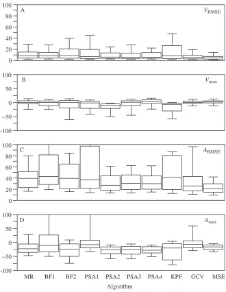
The distributions of VRMSE, Vmax, ARMSEand Amaxfor each
algorithm, pooled across sample, VM and VS, are summarized using box plots (Fig. 2). In these plots, the median is a measure of a method’s tendency, while the error variation (the variance of the errors around zero and not around the distribution’s mean or median) is a measure of a method’s robustness or ability to avoid large errors. Differences in the pooled distributions among algorithms were relatively small for the velocity but large for the acceleration measures. For VRMSE,
the median estimates differed trivially but the distributions of BF2, PSA1 and KPF were positively skewed, indicating less robustness. In contrast, GCV and, especially, MSE were the most robust algorithms for estimates of the entire velocity history over the range of VM and VS simulated here. For Vmax,
the MR, BF1, PSA4, GCV and MSE algorithms had generally symmetrical distributions of small variance with slightly positive medians (<5 %). The negatively skewed distributions of BF2, PSA1–3 and KPF indicate a tendency to underestimate Vmax. Again, the two spline algorithms were the most robust.
As for the velocity estimates, the pooled distributions suggest that MSE and, to a lesser degree, GCV had a better global performance for acceleration estimates than did the other algorithms. For ARMSE, the MSE distribution not only had the
p y(m)(t)2d t
t1
tn
+ y (ti) – y (ti) 2
Σ
i =1 n
median with the smallest per cent error but also had the least positive skew, indicating its robustness. In contrast, the distribution of GCV had a relatively small median error but was highly positively skewed. Other methods that were prone to large errors were BF1, BF2, PSA1 and KPF. The distribution of Amaxindicates that all methods tend to underestimate maximum
accelerations. The three methods with the smallest median per cent error, BF1, PSA1 and GCV, were associated with highly positively skewed distributions. In contrast, the PSA2, PSA3, PSA4 and, especially, MSE algorithms had moderate to relatively large median errors but were far less likely to result in grossly incorrect estimates of maximum acceleration.
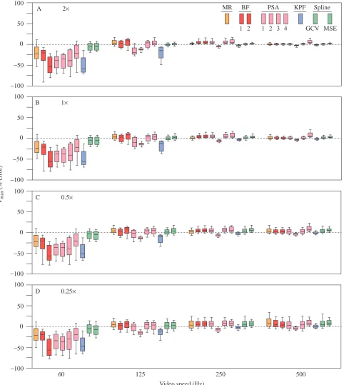
Local performance: effects of video magnification and speed The global error distributions (Fig. 2) fail to highlight the complex interactions between algorithm, VM and VS on algorithmic performance (Figs 3–6). The major features of the distributions of the performance measures within each VM×VS combination (Figs 3–6) are (1) the marked decrease in the
magnitude of both the median error and the error variance from 60 to 250 Hz and the slight (high VM) to large (low VM) increase in error from 250 to 500 Hz (especially conspicuous for the acceleration data), (2) the decrease in error with increasing VM, especially at high VS, and (3) the decrease in variance among methods from 60 to 250 Hz but the increase from 250 to 500 Hz, a pattern that was particularly conspicuous at low VM. There were exceptions to 1: throughout the increase in VS, both the maximum and RMSE performances of MSE and KPF improved, the RMSE performances of PSA1–4 improved and the acceleration performances of GCV worsened.
For VRMSE (Fig. 3), the two spline methods were clearly
superior at 60 Hz. At 125 Hz, the MR, BF2 and, especially, PSA1 and KPF algorithms performed the worst at the highest VM, but differences among methods became increasingly trivial as VM decreased. In contrast, for both 250 and 500 Hz, differences among algorithms were trivial at the highest VM but were increasingly large as VM decreased. At 500 Hz and 0.25×
MSE
MR BF1 BF2 PSA1 PSA2 PSA3 PSA4 KPF GCV
A VRMSE 100
80
60
40
20
0
D Amax 100
−100 0 50
−50
Per cent error
100
80
60
40
20
0
B Vmax 100
−100 0 50
−50
C ARMSE
[image:6.609.230.560.73.499.2]Algorithm Fig. 2. Box plot representations of the
distributions of the per cent errors for (A)
VRMSE, (B) Vmax, (C) ARMSEand (D) Amax.
The plot for each algorithm (see abbreviations in Table 1) summarizes the distribution of the errors pooled across the five displacement profiles of Harper and Blake (1991), the four levels of video magnification (VM), the four levels of video speed (VS) and the 100 resampled displacements for each combination of
profile×VM×VS. The box represents the
twenty-fifth and seventy-fifth percentiles. The line within the box is located at the distribution’s median. The lines (or whiskers) extending from the box mark the
tenth and ninetieth percentiles. VRMSE and
ARMSE are the per cent root mean square
error of the velocity and acceleration estimates, taken with respect to the true velocities and accelerations, for the middle 80 % of the sampled times within the
sequence. Vmax and Amax are per cent
magnification, the MR, BF1 and GCV algorithms performed the worst. The general patterns occurring in the distributions of VRMSEalso occurred in the distributions of Vmax (Fig. 4). At 60
and 125 Hz, the two spline algorithms had both the smallest
median errors and the smallest error variances, especially at high VM. The KPF method performed poorly at low VS but the best at high VS, particularly at high VM.
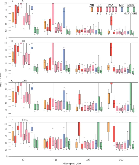
For both ARMSE (Fig. 5) and Amax (Fig. 6), the two spline
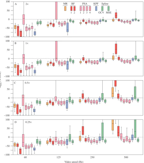
MR BF PSA KPF
2
1 3 4
1 2 GCV MSE
Spline
60 125 250 500
Video speed (Hz)
A 2×
100
80
60
40
20
0
VRMSE
(
% error)
B 1×
100
80
60
40
20
0
C 0.5×
100
80
60
40
20
0
D 0.25× 100
80
60
40
20
[image:7.609.72.547.76.608.2]0
Fig. 3. Box plot representations of the distributions of the per cent errors for VRMSE pooled across the five profiles and 100 resampled
displacements for each combination of VM×VS. VRMSEis the per cent root mean square error of the velocity estimates, taken with respect to the
true velocities, for the middle 80 % of the sampled times within the sequence. (A) 2× magnification, (B) 1× magnification, (C) 0.5×
algorithms were clearly superior at 60 Hz, especially at high VM. While MSE continued to have the best performance with increasing VS for ARMSE, the KPF algorithm had the best
performance for Amaxat high VS. PSA1–4 had relatively good
performance at low VM for both ARMSE and Amax. The low
sharpening factor of PSA1 resulted in a highly unstable performance for both acceleration measures at 60 and 125 Hz but good performance, relative to the other PSA variants, for
MR BF PSA KPF
2
1 3 4
1 2 GCV MSE
Spline
60 125 250 500
Video speed (Hz)
A 2×
100
−100 0 50
−50
B 1×
100
−100 0 50
−50
C 0.5×
100
−100 0 50
−50
D 0.25× 100
−100 0 50
−50
Vmax
[image:8.609.62.544.75.614.2](% error)
Fig. 4. Box plot representations of the distributions of the per cent errors for Vmax pooled across the five profiles and 100 resampled
displacements for each combination of VM×VS. Vmaxis the per cent difference between the estimated and true value of the maximum velocity
for each sampled profile. (A) 2× magnification, (B) 1× magnification, (C) 0.5× magnification and (D) 0.25× magnification. VM is video
estimates of Amax(but not ARMSE) at 250 and 500 Hz. The MR
method performed relatively well for estimates of both maximum acceleration and the entire acceleration profile at
high VM and VS, and at high VM and moderate VS, but poorly at either low VS or at high VS and low VM. For ARMSE, BF1
performed better than BF2 at 60 and 125 Hz but worse at 250
MR BF PSA KPF
2
1 3 4
1 2 GCV MSE
Spline
60 125 250 500
Video speed (Hz)
A 2×
100
80
60
40
20
0
B 1×
100
80
60
40
20
0
C 0.5×
100
80
60
40
20
0
D 0.25× 100
80
60
40
20
0
ARMSE
[image:9.609.73.547.75.634.2]
(% error)
Fig. 5. Box plot representations of the distributions of the per cent errors for ARMSE pooled across the five profiles and 100 resampled
displacements for each combination of VM×VS. ARMSEis the per cent root mean square error of the acceleration estimates, taken with respect
to the true accelerations, for the middle 80 % of the sampled times within the sequence. (A) 2× magnification, (B) 1× magnification, (C) 0.5×
and 500 Hz. For Amax, BF1 performed better than BF2 at 60,
125 and 250 Hz. The better of BF1 and BF2 performed well, relative to the other algorithms, at 250 Hz but very poorly at lower and higher video speeds.
Discussion
Computer simulation experiments have proved to be a powerful means of evaluating alternative numerical methods over a specified parameter space (Rohlf et al. 1990; Oden and
MR BF PSA KPF
2
1 3 4
1 2 GCV MSE
Spline
60 125 250 500
Video speed (Hz)
A 2×
100
−100 0 50
−50
B 1×
100
−100 0 50
−50
C 0.5×
100
−100 0 50
−50
D 0.25× 100
−100 0 50
−50 Amax
[image:10.609.58.538.74.616.2](% error)
Fig. 6. Box plot representations of the distributions of the per cent errors for Amax pooled across the five profiles and 100 resampled
displacements for each combination of VM×VS. Amax is the percent difference between the estimated and true value of the maximum
acceleration for each sampled profile. (A) 2× magnification, (B) 1× magnification, (C) 0.5× magnification and (D) 0.25× magnification. VM is
Sokal, 1992; Martins and Garland, 1991). The comparison of numerical differentiation algorithms has a relatively long history but has generally been limited to qualitative comparisons of only a few model sequences (Zernicke et al. 1976; Pezzack et al. 1977; McLaughlin et al. 1977; Wood and Jennings, 1979; Cappozzo and Gazzani, 1983). Two recent simulation studies that have compared the performance of several numerical differentiation algorithms (Corradini et al. 1993; Giakas and Baltzopoulos, 1997a) are of limited use to anyone using high-speed video because of the low (50–100 Hz) sampling frequency. Additionally, while Giakas and Baltzopoulos (1997a) compared the performance for a large number of signals, they reported only the relative rankings among the algorithms and not the actual or per cent errors. The simulation in the present study, which compared the performance of ten algorithms across different combinations of video magnification and speed, was designed to lend some guidance to the choice of numerical differentiation algorithm for biologists investigating animal movement.
Before discussing the results, I want to emphasize several caveats of this analysis. (1) The simulated behavior was highly aperiodic and non-stationary, which may bias the results in favor of methods that do not assume a periodic or stationary signal (Woltring, 1985). Nevertheless, the relatively good performance of the PSA and KPF algorithms at high VS suggests that detrending and, if necessary, odd-extension are adequate for these data. Additionally, a comprehensive simulation of periodic signals should be undertaken to evaluate the performance of the spline methods with periodic data. (2) The optimal VS for an algorithm should not be considered absolute. Instead, the important comparative parameter should be some measure of the frequency of the signal’s inflection points, for the derivative order of interest, relative to sampling frequency. (3) With the exception of the MSE algorithm, I have intentionally treated the process of numerical differentiation as
a fully automatic methodology with no input of either subjective or objective external knowledge (the MSE algorithm differs from the others by employing an estimate of the measurement error). The wisdom of this approach is debatable, but these results do show that good estimates can occur in complete ignorance of either the processes generating the signal or the mechanics of the algorithms. (4) Woltring (1991) suggested that the optimal smoothing parameter may differ for derivatives of different order and that more smoothing may be necessary for higher-order derivatives (see also Hatze, 1981; Giakas and Baltzopoulos, 1997b). The smoothness of the derivatives investigated in the present study were determined by the measured function only (zeroth-order derivative). (5) Finally, this study explicitly simulated data derived from video which, in general, has far lower resolution than high-speed film. Film-derived data should therefore have smaller expected errors than video-derived data at comparable filming magnification and speed.
Comparative performance
The simulations reported here suggest that no method performs best across all regions of the VM×VS parameter space. This conclusion is not surprising and supports the findings of analyses that simulated data sampled at lower frequencies than those reported here (Corradini et al. 1993; Giakas and Baltzopoulos, 1997a). Because of the variation in rank-order performance with changes in VM and VS, the global performance statistics should be treated cautiously. Despite the caution about using a universal differentiator, the MSE quintic spline algorithm was highly stable over the entire parameter space simulated here and can be generally recommended. When outperformed by another algorithm, both the difference between the estimates and the error from the true value were very small. A potential, but unexplored, problem with the MSE algorithm is its sensitivity to misestimates of the input error.
Corradini et al. (1993) compared the second-derivative performance of five different numerical differentiators including a heptic spline version of MSE (the four other algorithms in their study were not investigated here). Five simulated functions sampled between 50 and 100 Hz were used for the analysis. Supporting the results reported here, Corradini et al. (1993) showed that the MSE algorithm performed better than the other four functions for estimates of the entire acceleration profile.
The GCV performed very well over much of the parameter space. For Amax, in particular, at least 50 % of the GCV
estimates had relatively small errors at nearly all combinations of VM and VS. At high VS, however, the GCV algorithm proved unstable, often resulting in severely overestimated velocity and acceleration estimates. This suggests that, in general, if the GCV acceleration profile does not look markedly noisy, the resulting estimates should be reasonable. It is somewhat surprising that GCV performed as well as it did at 60 and 125 Hz. Woltring (1985, 1986a) explicitly warned against using the GCV criterion on data sets with fewer than 40 points; in the present study, the ranges of sample sizes of
0 20 40 60 80
0 0.1 0.2 0.3 0.4
Acceleration (m s
−
2)
[image:11.609.78.269.73.261.2]Time (s)
the data at 60 and 125 Hz were 7–8 and 15–16 points, respectively.
Giakas and Baltzopoulos (1997a) recently compared GCV with five other algorithms including PSA3 and Winter’s (1990) residual analysis (RA) method of estimating the optimal Butterworth filter (similar in spirit to BF1 and BF2). Giakas and Baltzopoulos (1997a) evaluated the performance of the algorithms on data from 24 simulated signals sampled at 50 Hz with 30 different levels of added noise. Each signal was sampled only once for a level of added noise. Giakas and Baltzopoulos (1997a) reported global rankings only (i.e. pooled over noise level) for estimates of the whole profile and found PSA3 to have better performance than both GCV and RA for both velocity and acceleration estimates. Actual error levels were not reported, except for a single signal (which, curiously, showed GCV performing better than PSA3 for nearly all levels of added noise).
The MR algorithm is a commonly used method for estimating accelerations in the animal locomotion literature, especially for measures of fast-start performance (Webb, 1977, 1978; Domenici and Blake, 1991, 1993; Kasapi et al. 1993; Law and Blake, 1996). While the MR algorithm performed well for estimating velocities for data sampled at or above 125 Hz, it only performed well for estimates of acceleration at 250 Hz. At lower sampling frequencies, the MR algorithm severely underestimated accelerations; at higher frequencies, it severely overestimated accelerations.
To stabilize edge effects at the beginning and end of a sequence, D’Amico and Ferrigno (1990, 1992) used forward and backward linear prediction to extend the observed sequence prior to filtering. While my implementation of the linear prediction extension worked well for the well-known displacement data of Pezzack et al. (1977), unusually large errors at the ends occurred for many of the simulated sequences analyzed in the present study. My use of quadratic polynomial regression to extend the data resulted in edges with less error than occurred with the linear prediction extension. In their exploration of the PSA differentiator, D’Amico and Ferrigno (1990, 1992) varied the magnitude of the sharpening factor (see Materials and methods) between 1 and 5 and concluded that a value of 1 was best if acceleration maxima are desired but a value of 2–3 tended to minimize the RMSE. D’Amico and Ferrigno’s (1992) conclusion is supported for the simulated fast-start data analyzed here; PSA1, with a sharpening factor of 1, performed much better than the other PSA algorithms for Amax. Indeed, PSA1 was one of the best
methods for Amax at low VM and high VS. PSA2–4 all
performed similarly, except that PSA3–4 had smaller errors at the edges than did PSA2 (this result is not apparent in the RMSE figures since only the intermediate 80 % of the points were used for the calculation of RMSE).
Lanczos’ moving regression (MR) method
The use of numerical differentiation to estimate maximum acceleration was criticized by Harper and Blake (1989), who showed that estimates using typical film speeds (250 Hz) and
magnification have an expected error of approximately 40 %. Such high errors certainly preclude reasonable reconstruction of locomotor dynamics or comparisons of acceleration performance. Harper and Blake (1989) recognized two sources of errors: sampling frequency error (SFE) and measurement error (ME). While the presence of these errors is inherent in numerical differentiation, their influence on derivative estimates can be minimized by the selection of an appropriate numerical differentiator. Harper and Blake (1989), following Webb (1977, 1978), used Lanczos’ moving regression (MR) algorithm to estimate accelerations (Lanczos, 1956). The pattern of the error distributions for the MR algorithm observed in this study (Figs 3–6), that is, an initial decrease and final increase in per cent error, with increasing VS, closely resembles the expected pattern discussed by Harper and Blake (1989).
A major advantage of the MR algorithm is that it is computationally trivial, while its chief disadvantage is that it does not allow the user to control the degree of smoothing [see Lanshammar (1982a) for a more flexible use of piecewise polynomials]. The second derivative of a quadratic polynomial is constant and, if the function’s second derivative varies, the computed second derivative will be a weighted average of the function’s second derivatives at each of the points used to estimate it. As a consequence, estimates of the maximum second derivative of a function sampled without noise will always be too low. Harper and Blake (1989) refer to this source of error as sampling frequency error because, as the function is sampled at smaller intervals, variation in the function’s second derivative at any five neighboring points becomes increasingly smaller, and the polynomial’s second derivative will approach that of the sampled function.
Harper and Blake (1989) argued that the measurement error component of the total error in estimating maximum accelerations increases with increasing film speed because digitizing error, although constant in magnitude, increases relative to the distance moved by the animal between successive frames. As a result, the total error increases at speeds above the optimum (Harper and Blake, 1989). This argument is contrary to the analysis of derivative errors by Lanshammar (1982b), who suggested that errors will continually decrease with increasing VS. Harper and Blake’s (1989) argument may explain the extreme overestimation of Amaxfor the MR algorithm at 500 Hz when VM was ⭐0.5×. In
addition to MR, the BF1, BF2 and GCV algorithms also markedly overestimated maximum accelerations at high VS. Importantly, however, some algorithms were resistant to this source of error, at least at the video speeds and magnitudes analyzed in this study. PSA2, PSA4 and MSE nearly always underestimated maximum accelerations, and the magnitude of this underestimation decreased with VS. PSA1, PSA3 and KPF often overestimated maximum accelerations at high but not at low VS but, again, the absolute error decreased with increasing VS, at least up to 500 Hz. The results of the present study, then, show that changes in error, with respect to VS, are more complicated than suggested by either Harper and Blake (1989) or Lanshammar (1982b).
How to get better results
The performance of the automated differentiating algorithms over the parameter space simulated in this study suggests a more optimistic role for numerical differentiation in studies of comparative performance and locomotor dynamics than concluded by Harper and Blake (1989). Two properties are important when choosing a numerical differentiator: the expected performance of an algorithm and the robustness of the algorithm. The expected performance, represented in this study by an algorithm’s median performance, measures the
bias of an algorithm. For example, the MSE algorithm consistently underestimates the actual maximum acceleration. If enough were known about this bias, a correction factor could be added to estimates of Amax. One caveat to using such a
correction factor is that not only does the magnitude of the bias vary with VM and VS but it should also vary with the shape of the displacement profile (the effects of which were not measured in this study).
Perhaps more important for comparative performance analyses is an algorithm’s robustness, represented by the error variance of the performance estimates. For example, the median per cent error for Amaxby the GCV algorithm at 500 Hz
and 1× magnitude was only −0.3 %, but more than 10 % of the estimates were overestimated by over 100 %. In contrast, the MSE algorithm had a slightly higher median per cent error (−9.5 %) but a much smaller error variance. As a result, although the MSE may underestimate the actual maximum acceleration, it should underestimate the maximum by a similar magnitude for all individuals.
The results of the video data presented here suggest that even the best numerical differentiation algorithms may result in error variation large enough to preclude comparisons of subtle performance variation. For example, the large errors associated with the MR and GCV algorithms at high VS may explain the failure to find significant differences in maximum acceleration between closely related fish using film data and the MR algorithm (Law and Blake, 1996) or between samples subjected to different treatments using video data and the GCV algorithm (Beddow et al. 1995). Because film data allows much higher resolution than video, error variances should be minimized when using the KPF, PSA, GCV or MSE algorithms in combination with high-speed film.
While the RMSE associated with estimating velocity profiles was low, it was uncomfortably high for the acceleration profiles (the best performers had error rates of 11.1 % at 500 Hz and 2×and 27.0 % at 500 Hz and 0.25×). It is well known that numerical differentiators are highly unstable at the edges of a sequence. Some of these methods attempted to control for this by artificially extending the sequence either after (KPF) or before and after (BF, PSA) the original sequence. Nevertheless, edge effects were apparent (the reason why the measure of RMSE included only the intermediate 80 % of the points). Clearly, there is no substitute for actual measurements of displacement before and after the sequence of interest. Additionally, if using the GCV spline, the added points should increase the accuracy of the estimate of the optimal smoothing parameter.
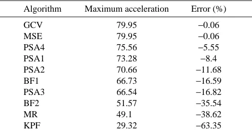
[image:13.609.49.298.109.241.2]Given the large amount of data in this study, I did not explore the causal explanation of the high RMSE; that is, if the general pattern of peaks and troughs present in the true acceleration profile was faithfully reconstructed despite the large RMSE or if the entire shape of the profile was incorrectly estimated. This is an important distinction because completely misshapen estimates of acceleration profiles could lead to highly inaccurate dynamic models of animal movement. A useful addition for future simulations would be to explore Table 2. Estimates of maximum acceleration and their per
cent error for the function in Fig. 7 sampled at 60 Hz without added noise
Algorithm Maximum acceleration Error (%)
GCV 79.95 −0.06
MSE 79.95 −0.06
PSA4 75.56 −5.55
PSA1 73.28 −8.4
PSA2 70.66 −11.68
BF1 66.73 −16.59
PSA3 66.54 −16.82
BF2 51.57 −35.54
MR 49.1 −38.62
KPF 29.32 −63.35
The true maximum acceleration was 80.0 m s−2. Because no noise
was added to the sampled points, the error reflects underestimation of the maximum acceleration due to oversmoothing.
correlates of algorithmic performance. For example, do we have more confidence in an estimate if all algorithms give similar values? Similarly, numerically estimated acceleration profiles of the center of mass during steady swimming in a fish showed little variation within swimming speed, either among sequences or among individuals (Walker and Westneat, 1997). Does the similarity in these sequences indicate good estimates of the acceleration profile or were all of the profiles incorrectly estimated in the same way? Additional simulations could investigate whether we should have more confidence in our numerically differentiated results, given a similarity in profile shapes.
Finally, time-averaged performance measures have been suggested as alternatives to instantaneous estimates in order to avoid the potentially large errors resulting from numerical differentiation. Indeed, many studies of fast-start performance report only the total distance travelled in some behavior or a velocity based on this distance and the duration of the travel (Webb and Skadsen, 1980; Taylor and McPhail, 1986; Eaton et al. 1988; Jayne and Bennett, 1990; Norton, 1991; Swain, 1992; Watkins, 1996). While time-averaged measures of performance do not suffer from exponentially magnified error propagation, they do suffer from masking proximate explanations of performance variation. Many of the critical features of the acceleration profiles measured by Harper and Blake (1990, 1991), including time to peak acceleration and number of acceleration peaks, could not have been discovered using time-averaged performance measures. More importantly for studies of comparative performance, the variation in acceleration profiles among individual fast starts (Harper and Blake, 1990, 1991) demonstrates the complex relationship between the distance traveled during some arbitrary time and maximum acceleration. This complex relationship suggests that time-averaged measures of fast-start performance may not be a good indicator of acceleration performance. Inter-individual and intra-Inter-individual escape behaviors are highly variable and context-dependent (e.g. Huntingford et al. 1994). It seems likely that both high initial accelerations (e.g. rapid jumps) and high average velocities (e.g. escapes into a refuge) can be closely related to survival, but the relative influence of each may depend on the context of the response. Because of both the complexity of fast-start movements and the variation in escape behavior, time-averaged measures cannot replace instantaneous measures of escape performance.
I thank Will Corning, Nora Espinoza, Melina Hale, Mark Westneat, Brad Wright and two anonymous reviewers for greatly improving the manuscript. This research was performed while on the generous support of a National Science Foundation Postdoctoral Research Fellowship in the Biosciences Related to the Environment.
References
BEDDOW, T. A., VANLEEUWEN, J. L. ANDJOHNSTON, I. A. (1995).
Swimming kinematics of fast starts are altered by temperature
acclimation in the marine fish Myoxocephalus scorpius. J. exp. Biol. 198, 203–208.
CAPPELLO, A., LA PALOMBARA, P. F. AND LEARDINI, A. (1996).
Optimization and smoothing techniques in movement analysis. Int. J. bio-med. Comput. 41, 137–151.
CAPPOZZO, A. AND GAZZANI, F. (1983). Comparative evaluation of
techniques for the harmonic analysis of human motion data. J. Biomech. 16, 767–776.
CORRADINI, M. L., FIORETTI, S. AND LEO, T. (1993). Numerical
differentiation in movement analysis: how to standardise the evaluation of techniques. Med. Biol. Eng. Comput. 31, 187–197.
CRAVEN, P. ANDWAHBA, G. (1979). Smoothing noisy data with spline
functions. Estimating the degree of smoothing by the method of generalized cross-validation. Numer. Math. 31, 377–403.
D’AMICO, M. ANDFERRIGNO, G. (1990). Technique for the evaluation
of derivatives from noisy biomechanical displacement data using a model-based bandwidth-selection procedure. Med. Biol. Eng. Comput. 28, 407–415.
D’AMICO, M. AND FERRIGNO, G. (1992). Comparison between the
more recent techniques for smoothing and derivative assessment in biomechanics. Med. Biol. Eng. Comput. 30, 193–204.
DENNY, M. W. (1988). Biology and the Mechanics of the Wave-Swept Environment. Princeton: Princeton University Press.
DOMENICI, P. AND BLAKE, R. W. (1991). The kinematics and
performance of the escape response in the angelfish (Pterophyllum eimekei). J. exp. Biol. 156, 187–205.
DOMENICI, P. AND BLAKE, R. W. (1993). The effect of size on the
kinematics and performance of angelfish (Pterophyllum eimekei) escape responses. Can. J. Zool. 71, 2319–2326.
EATON, R. C., DIDOMENICO, R. AND NISSANOV, J. (1988). Flexible
body dynamics of the goldfish C-start: implications for reticulospinal command mechanisms. J. Neurosci. 8, 2758–2768. GAZZANI, F. (1994). Comparative assessment of some algorithms for
differentiating noisy biomechanical data. Int. J. bio-med. Comput. 37, 57–76.
GIAKAS, G. AND BALTZOPOULOS, V. (1997a). A comparison of
automatic filtering techniques applied to biomechanical walking data. J. Biomech. 30, 847–850.
GIAKAS, G. ANDBALTZOPOULOS, V. (1997b). Optimal digital filtering
requires a different cut-off frequency strategy for the determination of the higher derivatives. J. Biomech. 30, 851–855.
HARPER, D. G. ANDBLAKE, R. W. (1989). A critical analysis of the
use of high-speed film to determine maximum accelerations of fish. J. exp. Biol. 142, 465–471.
HARPER, D. G. ANDBLAKE, R. W. (1990). Fast-start performance of
rainbow trout Salmo gairdneri and northern pike Esox lucius. J. exp. Biol. 150, 321–342.
HARPER, D. G. ANDBLAKE, R. W. (1991). Prey capture and the
fast-start performance of northern pike Esox lucius. J. exp. Biol. 155, 175–192.
HATZE, H. (1981). The use of optimally regularized Fourier series for estimating higher-order derivatives of noisy biomechanical data. J. Biomech. 14, 13–18.
HUNTINGFORD, F. A., WRIGHT, P. J. AND TIERNEY, J. F. (1994).
Adaptive variation in antipredator behavior in threespine stickleback. In Evolutionary Biology of the Threespine Stickleback (ed. M. A. Bell and S. A. Foster), pp. 277–296. Oxford: Oxford University Press.
JAYNE, B. C. AND BENNETT, A. F. (1990). Selection on locomotor
KASAPI, M. A., DOMENICI, P., BLAKE, R. W. ANDHARPER, D. (1993). The kinematics and performance of escape responses of the knifefish Xenomystus nigri. Can. J. Zool. 71, 189–195.
LANCZOS, C. (1956). Applied Analysis. London: Isaac Pitman & Sons (reprinted 1988; New York: Dover).
LANSHAMMAR, H. (1982a). On practical evaluation of differentiation techniques for human gait analysis. J. Biomech. 15, 99–105. LANSHAMMAR, H. (1982b). On precision limits for derivatives
numerically calculated from noisy data. J. Biomech. 15, 459–470.
LAW, T. C. AND BLAKE, R. W. (1996). Comparison of fast-start
performances of closely related, morphologically distinct threespine sticklebacks (Gasterosteus spp.). J. exp. Biol. 199, 2595–2604.
MARTINS, E. P. ANDGARLAND, T., JR(1991). Phylogenetic analysis
of the correlated evolution of continuous characters: a simulation study. Evolution 45, 534–557.
MCLAUGHLIN, T. M., DILLMAN, C. J. AND LARDNER, T. J. (1977).
Biomechanical analysis with cubic spline functions. Res. Quart. 48, 569–582.
NIKLAS, K. J. (1992). Plant Biomechanics. Chicago: University of Chicago Press.
NORBERG, U. M. (1990). Vertebrate Flight. Berlin: Springer-Verlag. NORTON, S. F. (1991). Capture success and diet of cottid fishes: the
role of predator morphology and attack kinematics. Ecology 72, 1807–1819.
ODEN, N. L. AND SOKAL, R. R. (1992). An investigation of
three-matrix permutation tests. J. Class. 9, 275–290.
PEZZACK, J. C., NORMAN, R. W. AND WINTER, D. A. (1977). An
assessment of derivative determining techniques used for motion analysis. J. Biomech. 10, 377–382.
RAYNER, J. M. V. AND ALDRIDGE, H. D. J. N. (1985).
Three-dimensional reconstruction of animal flight paths and the turning flight of microchiropteran bats. J. exp. Biol. 118, 247–265.
ROHLF, F. J., CHANG, W. S., SOKAL, R. R. AND KIM, J. (1990).
Accuracy of estimate phylogenies: Effects of tree topology and evolutionary model. Evolution 44, 1671–1684.
SMITH, G. (1989). Padding point extrapolation techniques for the Butterworth digital filter. J. Biomech. 22, 967–971.
SWAIN, D. P. (1992). The functional basis of natural selection for vertebral traits of larvae in the stickleback Gasterosteus aculeatus. Evolution 46, 987–997.
TAYLOR, E. B. AND MCPHAIL, J. D. (1986). Prolonged and burst
swimming in anadromous and freshwater threespine stickleback, Gasterosteus aculeatus. Can. J. Zool. 64, 416–420.
VOGEL, S. (1994). Life in Moving Fluids (2nd edn). Princeton: Princeton University Press.
WAINWRIGHT, P. C. AND REILLY, S. M. (1994). Ecological
Morphology. Chicago: University of Chicago Press.
WALKER, J. A. (1997). QuickSAND. Quick Smoothing and Numerical Differentiation for the Power Macintosh. [WWW Document. URL http://jaw.fmnh.org/software/qs.html.]
WALKER, J. A. ANDWESTNEAT, M. W. (1997). Labriform propulsion
in fishes: kinematics of flapping aquatic flight in the bird wrasse Gomphosus varius (Labridae). J. exp. Biol. 200, 1549–1569. WATKINS, T. B. (1996). Predator-mediated selection on burst
swimming performance in tadpoles of the Pacific tree frog, Pseudacris regilla. Physiol. Zool. 69, 154–167.
WEBB, P. W. (1977). Effects of median-fin amputation on fast-start performance of rainbow trout (Salmo gairdneri). J. exp. Biol. 68, 123–135.
WEBB, P. W. (1978). Fast-start performance and body form in seven species of teleost fish. J. exp. Biol. 74, 211–226.
WEBB, P. W. (1982). Locomotor patterns in the evolution of actinopterygian fishes. Am. Zool. 22, 329–342.
WEBB, P. W. (1984). Body form, locomotion and foraging in aquatic vertebrates. Am. Zool. 24, 107–120.
WEBB, P. W. ANDSKADSEN, J. M. (1980). Strike tactics of Esox. Can.
J. Zool. 58, 1462–1469.
WINTER, D. A. (1990). Biomechanics and Motor Control of Human Movement. New York: John Wiley & Sons.
WOLTRING, H. J. (1985). On optimal smoothing and derivative estimation from noisy displacement data in biomechanics. Hum. Movmt Sci. 4, 229–245.
WOLTRING, H. J. (1986a). A Fortran package for generalized, cross-validatory spline smoothing and differentiation. Adv. Eng. Software 8, 104–107.
WOLTRING, H. J. (1986b). GCVSPL. [WWW Document. URL http://www.netlib.org/gcv/gcvspl.]
WOLTRING, H. J. (1991). Review and rebuttal. E-mail to biomech-l, 24 February, 1991.
WOOD, G. A. (1982). Data smoothing and differentiation procedures in biomechanics. Exercise Sport Sci. Rev. 10, 308–362.
WOOD, G. A. AND JENNINGS, L. S. (1979). On the use of spline
functions for data smoothing. J. Biomech. 12, 477–479.
ZERNICKE, R. F., CALDWELL, G. ANDROBERTS, E. M. (1976). Fitting