An analysis of type F2 software measurement standards for profile surface texture parameters

An analysis of Type F2 software measurement standards for

profile surface texture parameters

L D Todhunter1, R K Leach1, S D A Lawes1and F Blateyron2

1_{Manufacturing Metrology Team, Faculty of Engineering, University of}

Notting-ham, UK

2_{Digital Surf, Besançon, France}

Abstract. This paper reports on an in-depth analysis of ISO 5436 part 2 type F2

ref-erence software for the calculation of profile surface texture parameters that has been

performed on the input, implementation and output results of the reference software

de-veloped by the National Physical Laboratory (NPL), the National Institute of Standards

and Technology (NIST) and Physikalisch-Technische Bundesanstalt (PTB). Surface

tex-ture parameters have been calculated for a selection of seventeen test data files obtained

from the type F1 reference data sets on offer from NPL and NIST. The surface texture

parameter calculation results show some disagreements between the software methods of

the National Metrology Institutes. These disagreements have been investigated further,

and some potential explanations are given.

KeywordsProfile surface texture parameters, software measurement standards.

1

Introduction

The need to measure surfaces in manufacturing stems from an increasing need for precise and accurate component control, both in terms of the geometry of the component’s surfaces and the surfaces’ ultimate function [1, 2]. As manufactured parts get more complex, the effect of their micro-scale attributes plays a more important role in their functional properties, with the surface of a component serving as the point of interaction between itself, other components and the environment [3]. The fine structure, or texture, of a surface can influence material properties such as durability [4, 5], and consequently there is an increasing need for greater surface control.

1.1

Surface texture parameters

surface texture parameters are defined in ISO 4287 [9]. Each parameter is given an identifier, description and mathematical definition. The mathematical operations required to determine a parameter from surface measurement data are performed computationally; using software packages with measurement instruments, or third-party alternatives. ISO 5436-2 introduced ’software measurement standards’, created with the intention of being as accurate as possible, in order to verify the results of a measurement software package [10]. Software measurement stan-dards come in two types: type F1 reference datasets with certified results, and type F2 reference software which calculate surface texture parameters for any input file.

These software measurement standards are produced by National Metrology Institutes (NMIs). Some of the most well regarded software measurement standards for surface texture are the fol-lowing: ’softgauges version 1.01’ produced by the National Physical Laboratory (NPL), UK, available athttp://resource.npl.co.uk/softgauges/Ref_Algo_Overview.htm[11, 12]; ’SMATS version 1.0’ produced by the National Institute of Standards and Technology (NIST), USA, available athttp://physics.nist.gov/VSC/jsp/index.jsp[13, 14, 15]; and ’RPTB version 2.06’ produced by Physikalisch-Technische Bundesanstalt (PTB), Germany, available athttps://www.ptb.de/rptb[16, 17].

With several NMIs producing reference software, it becomes necessary to compare them with each other to establish equivalence of the software measurement standards. The definitions laid out in the ISO 4287 and 5436-2 standards must be interpreted and adapted to software, and may be implemented in multiple ways, producing different results. Additionally, some ISO definitions may present ambiguity, leading to further variations in the end result. A good example of an ambiguity in the ISO definitions is shown in [18], where Leach and Harris reveal an ambiguity in the definition of profile element discrimination, which leads to the number of profile elements counted in a certain length to be unclear, producing different values for theRSm spacing parameter. The RSmambiguity is just one, fairly severe example of ambiguity in the parameter definitions1. It is expected that there are more ambiguities elsewhere in the ISO steps required to go from a primary profile to a surface texture parameter value.

1.2

Previous software comparisons

Comparison allows differences in the obtained parameter values to be discovered, giving the potential to highlight ambiguities in the ISO specification standards in the hope that they may be better defined. Research carried out by Baker et al. [20] and Koenders et al. [21] performed comparisons between many laboratories across the world, obtaining roughness parameters for a variety of different physical measurement standards. These comparisons highlighted theRSm parameter variations mentioned by Leach and Harris. In 2009, Li et al. [22] focussed more on

the in-house software offerings of NPL, PTB and NIST, along with three commercial software packages. Li’s report went into further detail about the software packages, identifying some differences in software implementation. For example, Li et al. highlighted that NPL uses in-terpolation of the input data points to create a continuous profile, whereas PTB and NIST work with a discrete profile. Li et al. performed their comparison with six type F1 reference data sets, again finding generally good agreement between the NMIs. The software measurement stan-dard comparison used the PTB software ’RTPB v1.05’, which has since been updated, bringing the values obtained by PTB much closer to those obtained by NPL and NIST, particularly for the average ordinate parameters (Ra,Rq, etc.). Li et al.’s work also highlighted the increased dis-agreement forRSmvalues and the need for a better definition for this parameter, along with the Rcparameter. More recently, Paricio et al. [23] performed a similar experiment, comparing the software on offer from NPL, PTB and NIST. Paricio’s work had a greater focus on the user side of the software, commenting on the usability for the end-user. The comparison was performed using data files created in-house, from rectilinear sections. The results showed good agreement for a small selection of profile and roughness parameters, with PTB’s results differing slightly from NPL and NIST, showing a tendency to provide smaller values.

1.3

In-depth comparison

While it is clear that comparisons of NMI parameter calculation software have been carried out before, there is potential to delve deeper into the results obtained, whereby a comparison is made with equal focus on parameter results and software implementation, enabling the op-portunity for links to be made between the two. Such work has the potential to highlight how subtle differences in implementation of type F2 software measurement standards affect calcu-lated parameter values. A comparison of this nature could identify areas of the ISO specification standards which require clearer definitions to avoid ambiguity.

The aim of the work presented in this paper is to perform an in-depth analysis of the type F2 software measurement standards available from NPL, PTB and NIST. This analysis will com-prise both a comparison of the parameter values produced by each NMI software for a selection of test files, and an investigation into the differences in implementation of the standards, work-flow routes and default settings chosen by each of the NMI software packages. The combination of the two aspects has the potential to allow any observed implementation differences to explain differences in the parameter results. While areal surface texture parameters have been produced [24], this paper focuses on profile surface texture parameters only due to their easier theory and wider use in industry.

measurement standards, discussing the different software choices in detail and the algorithmic flow of each software package. Section 3 provides a description of the experiment methodol-ogy, justifying the test data files used and the process of performing the comparison. Section 4 discusses the results of the profile surface texture parameter calculations. Finally, section 5 summarises the outcomes of the work and concludes the paper.

2

Implementation of software

2.1

Input file requirements

All three NMIs accept the .SMD file format, as defined in ISO 5436-2. NIST and PTB also accept .SDF files, which is the ISO-defined file-type for areal software measurement standards [25]. The .SDF format is a useful addition, as it allows profile and areal measurements to be pre-processed for parameter calculation in the same way, saving time for users of the software that use both measurement types. Additionally, the NIST software accepts the .TXT format, a common text file type, and PTB accepts the .PR filetype, a simplified version of the .SMD from an old Breitmeier UBM instrument. Although the NPL software is restricted to the SMD format, to facilitate a wider use of the software NPL provide a “data file converter” at http://161.

112.232.32/softgauges/Converter.aspxto include .SDF, .PRF and .TXT file formats. All three NMIs assume the height value points within the input file are uniformly spaced along the X-axis. Uniform spacing is part of the .SMD definition in ISO 5436-2, and allows for a much simpler analysis of the file. On top of uniform spacing, NPL assumes some initial processing has already been carried out. In line with the definitions in ISO 5436-2, the NPL software requires an input of a primary profile. Using a primary profile means the input file must already have had the form removed, and must be λs filtered, so that any wavelengths shorter than those associated with roughness are removed. NIST and PTB, however, have no such restrictions and include options for form removal andλsfiltering, allowing them to work with files with no prior processing undertaken.

2.2

Algorithm flow

To better understand software measurement standard implementation differences, it is necessary to determine the options each software package gives, including identifying all choices available to the user and highlighting the different paths that a user could take through the software.

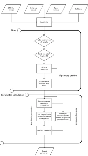
A good way to visualise the routes taken through the software is to create flow diagrams. The flow diagrams for NPL, PTB and NIST are given in Figures 10, 11 and 12, respectively, located toward the end of the paper due to their size. Each flow diagram shows the different software options and algorithmic routes that can be followed, along with inputs made by the user. On the PTB and NIST flow diagrams, a thick line is used to highlight the path through the software package that offers the greatest similarity to the NPL software package, which is useful for more direct comparison between NMIs. This is discussed in more detail in section 3.1. The software options filled in grey highlight any default settings in the software. What is immediately clear is the significant difference in complexity between the three software packages.

The NPL software is the simplest of the three. Once the file is input, there are only two sections to the software: λcFilter and Parameter Calculations - all that is required according to ISO 5436-2. The NPL software has no user options; once the file is chosen, the process is autonomous and the parameter values are calculated. This simplicity keeps the software package streamlined; its scope is accurately defined to match the requirements of a type F2 software measurement standard according to ISO 5436-2, and the software avoids the added complexity of additional features that can introduce further error or ambiguity. Whilst a single route ensures all parameter values are obtained through the same method and a good adherence to the ISO 5436-2 definitions, it is not very flexible, and should another filtration method be more suitable for a particular file, there is no way to take advantage of that. The filter used by the software is a linear Gaussian convolution, as defined in [7]. Following the filtration, the data is interpolated to form a continuous representation using a natural cubic spline [26]. The software uses this continuous representation to evaluate the parameters using the exact integral forms given in ISO 4287. For the waviness and roughness profiles, a length ofλcis removed from each end of the profile to avoid any end effects that may be caused by the filter application. Following parameter calculation, the user can choose the output format of the parameter values; either a .SMD file or .HTML file.

material ratio parameters. These filters include Gaussian convolution [7], Gaussian regression [27], Gaussian with end effect management [28] and spline filters [29]. This amount of choice makes for a very flexible system, but potentially adds confusion for inexperienced users. Fol-lowing the filtration, the choices become more limited. Users are able to select which parameter values are exported, along with certain inputs such as height/spacing discrimination values. The user can also choose the algorithm with which to calculate the material ratio parameters, which are not included in the NPL software. Following these parameter choices and their calculation, the results can be exported in .CSV file format and a .PDF report. During the filtration step of the software, the data is shown to the user visually, along with all obtained profiles. A vi-sual representation of the data is a useful addition, as seeing the data allows for a much better understanding, compared to a long dataset of raw values.

The NIST software at first looks highly complex, however, closer inspection reveals that the choices available to the user are relatively simple; there are instead more optional steps fol-lowing the parameter calculations. First, the user has the option of not only choosing their own data file to run through the software, but also a reference data file from NIST’s database. The ability to load files straight from the NIST database makes it easier for users who are using a NIST type F1 data file with their own software, as they can run the same file through the NIST software without having to download the file first. The user interface for the NIST software uses click-able tabs along the top of the window for selecting different sections of the software, allowing user control over which operations are performed. Additional sections in the software include power spectral density calculation, autocorrelation/cross-correlation and bearing-area-curve determination. Each of these additional sections come with simple choices to the user, such as the profile on which to operate and which method to use. As with PTB, NIST includes optional form removal andλsfiltering. Forλcfiltering, the choices are more limited than those given by PTB. The user can choose between Gaussian or 2RC filter methods; 2RC choices are between recursive and convolution methods, whereas Gaussian methods are between convolu-tion, ’Fast Gaussian’ and fast Fourier transform. For the Gaussian methods, the user can also choose whether to use a±0.5λcor±λcGaussian window, which dictates how large the cut-off regions are for the roughness and waviness profiles. Similar to PTB, the NIST software also shows the input data visually, albeit at a lower resolution.

3

Comparison methodology

3.1

Software choices for greatest comparability

Choos-ing similar options for each software package will minimise the number of potential sources of variation and make it easier to investigate any differences that do arise.

As the NPL software has only one algorithmic route available, it makes sense to choose options in the other two software packages to best match the steps taken by NPL. The software route includes the following:

1. The input data given is a primary profile; it must have form removed and beλsfiltered prior to input into the software.

2. Theλcfiltration shall be performed by a Gaussian convolution, as described in ISO 16610-21.

3. The parameters shall be calculated with the definitions given in ISO 4287.

4. For parameters that require height/spacing discrimination, a height discrimination of10% ofXz(the sum of the height of the largest peak and lowest valley within a sampling length, ISO 4287) and spacing discrimination of1% of the sampling length will be used. These are the default values as defined in ISO 4287.

5. If possible, no additional steps shall occur.

For point four in the list above, the discrimination values of10% ofXzand1% of the sam-pling length are taken from sections 4.1.4 and 4.3.1 in ISO 4287. This definition presents some ambiguity, as it can be interpreted as±5% around the mean line,±10% around the mean line, or10% of the peak-to-valley height in a profile element. It is unknown how each of the NMIs have interpreted this definition, and so theXzdiscrimination value may be a source of potential differences in the parameter results.

The closest routes through the NIST and PTB software are shown by the thick lines on the flow diagrams in Figures 12 and 11. For both NIST and PTB, it was possible to avoid extra steps, such as form removal andλsfiltering. The NIST software, being tabular in nature, allowed the selection of only the λcfiltering and parameter calculation steps. The PTB software is more sequential than the NPL software, forcing users to go through all steps of the software including material ratio parameter calculations, which are not required in this comparison, as the NPL software does not calculate them. However, while material ratio parameter calculations added time to the processing of the data files, it did not affect the filtration or values of the other parameters.

NPL. Both NIST and PTB also allowed the selection of the same ISO 4287 parameters that NPL calculates. Combined, these options allow for pathways through the software packages that are sufficiently close to allow a meaningful comparison. As mentioned above, the software options filled in with grey lines show the default choices in the software. These do not always match the NPL software, for example by having a form removal method enabled by default, or a different filter method selected that doesn’t match the suggested method from the ISO specification stan-dards. These differences mean selections must be actively changed by the user to obtain results comparable to another NMI, making it harder for a layman to get comparable results.

3.1.1 Sampling length ambiguity

ISO 4288 defines the evaluation length for the roughness profile to be built from a total of five sampling lengths, where each sampling length is equal to the length ofλc. However, ISO 4288 does not specify from where the sampling lengths will be taken if the profile length is longer than 5λc. The NPL software chooses to take the five sampling lengths from the centre of the profile, but it is not known whether NIST and PTB choose to do the same. This lack of guidance in the specification standards is another source of ambiguity than can lead to different parameter results, as the NMI software packages may be calculating the parameter values from sampling lengths with different starting points.

3.2

Choice of test files

With the software routes understood, a selection of test data files can be chosen to run through the software to compare the values. To make the comparison as useful as possible, the test files should be chosen to ensure a wide variety of profile types. The aim of the file selection is to test various aspects of parameter calculation, and identify the situations where differences may occur. The test files should include variations such as:

• Profile frequency- The density of the peaks and valleys of the profiles.

• Periodicity- The repeatability of the profile elements. Profiles that display a repeatable pattern have high periodicity; profiles that show significant variation between profile el-ements have low periodicity.

• Master piece profiles - Profiles that are taken from real surfaces and represent realistic surface finishes e.g. polished, ground.

• Profile amplitude- The height values of the peaks and valleys.

• Profile source- The location from which the profiles were obtained.

The test files used were type F1 reference data files taken from both NPL and NIST. Tak-ing files from NIST and NPL type F1 databases ensures the test files used come from reliable sources, and allows the test to be repeatable by anyone. In order to comply with the input re-quirements of NPL, primary profiles must be used. The NPL datasets were assumed to already comply with their own software requirements, however, this proved to be a false assumption, as discussed in section 4.5.1. Although the NIST datasets are by default given as total profiles, primary profiles are included in the downloadable .ZIP folder. From the full list of data files, seventeen test files were selected, ten from NPL and seven from NIST, which exhibit a variety of profile characteristics from the list above. The chosen files are shown in Figure 13.

3.3

Running files through the software

When attempting to input the files into the different software packages, some errors were found.

3.3.1 NIST input file issues

ISO 5436-2 defines the standard file-type for profile datasets to be .SMD [10]. ISO 5436-2 also gives a description of how the file should be structured, including the different records in the file and what they should contain. ISO 5436-2 also defines that each line, record and file should be ended with specific control characters, which are ASCII characters used to give information to the software reading the file, and are not represented by any written symbol. As a result, most common text editors do not show these characters, and a more advanced program is needed to read or write them.

A further error was found in some of the NIST type F1 files. The files used were primary profiles from the total profiles listed in the NIST database. It appears that in recreating the .SMD files with the primary profile data values, the number of points in the profile were not recounted. For some files, a small number of points had been removed from the profile, perhaps due to an effect of the form removal orλsfilter. However, the first record in the .SMD file defines the number of points in the file, and this number had not been updated to the true number for the primary profile, and instead matched the number for the total profile. In order for these files to work, the number of points had to be recounted, and the first record in the .SMD updated.

3.3.2 NPL input requirements

Because the NPL software has no user input once the file has been selected, all settings and required information must be included in the .SMD file. The .SMD must include which param-eters to calculate, and theλcvalue for the Gaussian filter. While versions of the NPL datasets could be downloaded with this information already in the .SMD file, the NIST files did not. To make the NIST type F1 files ready for use with the NPL software, each file had to include these NPL software instructions. As including the software instructions edits the characters in the .SMD file; the checksum also had to be recalculated and updated for these files.

3.3.3 Software outputs

Each file was processed through each software package using the user options shown in Figures 10, 11 and 12. All files were run withλc= 0.8mm. Keepingλcfixed for all files had several benefits; it reduced the complexity of the experiment, was the default setting for the NPL down-loaded files, and allowed for potential effects to be seen for test files where λc = 0.8mm is outside the optimum value for the cut-off filter. Once all parameter calculations were complete, the next step was to extract the parameter values from the software in order to analyse them.

4

Results and analysis

Once the primary profile test files were suitably pre-processed to be used in each NMI reference software package, each file was run through the reference software packages and parameter val-ues were obtained. The parameter valval-ues showed good agreement between NMIs for a many of the profile parameters and test files. Examples of this include average ordinate parameters such as PaandRq, and roughness parameters in general. This is unsurprising, as these parameters are the most simply defined and hence leave little room for interpretation. Test files that were simulated and periodic in nature, such andsin1andsaw123, also showed generally good agree-ment across many parameters. However, some areas of interesting disagreeagree-ment were identified between the NMIs, and these are highlighted and discussed in the sections below.

4.1

PTB negative

Xv

parameter values

It was found that PTB displayed its Xv parameter values as negative. ISO 4287 defines the Xv parameters using the magnitude of the valley depth, thus making the negative result non-compliant with the definition2_{. For the following analysis, the magnitude of theXvvalues was} used and displayed.

4.2

NPL sharp step overestimation

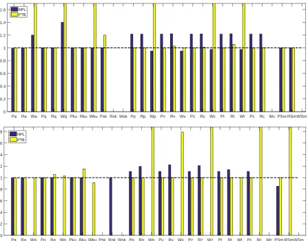
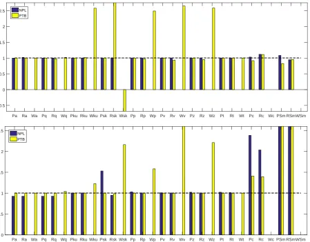
During the analysis it was found that, compared to the results obtained by NIST and PTB, the NPL software showed an overestimation for some parameter values. The overestimation was found mainly on peak/valley parameters, where no averaging of the ordinate values occurs, for test files that had very sharp steps. Some representative examples are given in Figure 1, which shows the relative parameter values for the squareandstepsfiles, with NIST as the arbitrarily chosen reference NMI. The relative parameter value graphs show the parameter values obtained by each software package normalised to unity for the reference NMI, given by

Xnnorm =

Xn Xnref N M I

, (1)

where Xn is the value of any surface texture parameter, Xnref N M I is the value of the same parameter for the chosen reference NMI and Xnnorm is the normalised value of the original parameter. As all normalised parameter values for the chosen reference are equal to one, their values are omitted from the graphs. Figure 1 shows that for both files, the Primary and Rough-ness peak/valley parameters obtained by NPL are around 20% larger than the values obtained

2_{This issue was brought to the attention of PTB, who have since updated their software to display the valley}

Pa Ra Wa Pq Rq Wq Pku Rku Wku Psk Rsk Wsk Pp Rp Wp Pv Rv Wv Pz Rz Wz Pt Rt Wt Pc Rc Wc PSm RSmWSm 0

0.2 0.4 0.6 0.8 1 1.2 1.4 1.6 NPL

PTB

Pa Ra Wa Pq Rq Wq Pku Rku Wku Psk Rsk Wsk Pp Rp Wp Pv Rv Wv Pz Rz Wz Pt Rt Wt Pc Rc Wc PSm RSmWSm 0

0.2 0.4 0.6 0.8 1 1.2 1.4 1.6 1.8

NPL PTB

Figure 1. Relative difference graphs for the square (top) and steps(bottom) test files. NIST

has been used as the comparison NMI. Overestimation is observed for P and R peak/valley parameters for the NPL results. The large values obtained by PTB shown here are due to another effect, and are discussed further in section 3

.

by the other two.

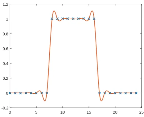
0 5 10 15 20 25 -0.2

0 0.2 0.4 0.6 0.8 1 1.2

Figure 2. A cubic spline used to fit a top-hat function. Oscillations around the step points are

clearly visible.

4.3

PTB large waviness values

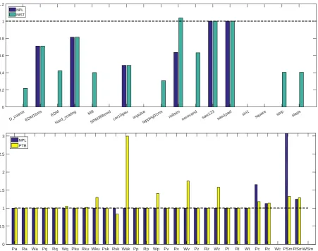
The PTB software was observed to obtain larger waviness parameter values than NPL and NIST, most prominently for some of the peak/valley parameters, occurring for almost all files. The larger waviness values were also present on some files for the average ordinate parameters (Wa, Wsk etc). Figure 3 gives examples of some of these, showing PTB in yellow giving larger waviness values than the other two. The top graph in Figure 3 shows theWpparameter in more detail, showing several files such asEDM16ms, Millandcor10gauwith much higherWpvalues. The bottom graph looks at theEDM16msfile specifically, and reveals that PTB obtained larger values than NIST and NPL for several waviness parameters, including Wv, Wz, WkuandWq. This effect is also shown in Figure 1, where PTB gives substantially larger values for several waviness parameters for both thesquareandstepstest files.

After discussions with PTB directly about the large waviness parameter values in comparison with NPL and NIST, it was discovered that PTB treat the ends of the waviness profile differently to NPL and NIST. In order to account for end effects, both NPL and NIST cut off the ends of the profile of lengthλc, and assess the remaining central portion. PTB, however, does not do this for the waviness profile. This causes the waviness profile to be longer and include more data points in the PTB software than the other two, leading to a greater chance of there being another peak (valley) with a high (low) value and resulting in a larger final parameter.

D_coarse EDM16ms EDM Hard_coating

Mill

SRM3filtered cor10gau impulse

lapping01ms millsim

normrand saw123 saw1pad sin1

square step steps

0 0.2 0.4 0.6 0.8 1 1.2

NPL NIST

Pa Ra Wa Pq Rq Wq Pku Rku Wku Psk Rsk Wsk Pp Rp Wp Pv Rv Wv Pz Rz Wz Pt Rt Wt Pc Rc Wc PSm RSmWSm 0

0.5 1 1.5 2 2.5 3

NPL PTB

Figure 3. Top: Relative values for theWpparameter for all files, normalised such than the PTB

of the feature being measured, and the roughness profile is equal to5λc. The waviness profile, however, has no such definition. ISO 4288 is, therefore, unclear as to whether the waviness profile length should be made similar to the roughness profile, or the primary profile. It appears that NIST and NPL have chosen to treat the waviness profile the same as the roughness profile, and PTB have decided to keep it the same length as the primary profile. It is speculated that this decision was made under the assumption that a profile should not be altered unless specifically stated in ISO specification standards3_.

4.4

NIST Wc and WSm failures

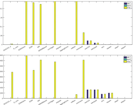
The NIST software was unable to obtain a value for Wcand WSmfor any test file, including its own reference data sets. Due to the nature of the calculation of WcandWSm, and the low amplitude of the waviness profile for many of the test files, it was anticipated that the software packages would struggle to obtain the values for all test files, however, not being able to obtain any is a notable issue. The result is shown in Figure 4, where PTB and NPL are shown to obtain values for some files, but NIST obtains none. It should be noted here that it is because of the WcandWSmfailures that there are no results shown forWcandWSmon any relative parameter value graph for which NIST is the reference NMI.

Upon further research into the implementation of these parameters by NIST, it was found in their ’help’ documentation that the height discrimination for the XcandXSm parameters is defined as a user set percentage of Rz. The ISO 4287 defines the height discrimination to use Xz, e.g. use Wz for Wc/WSm. The description of the height discrimination in the NIST doc-umentation could simply be poorly worded, however, if the docdoc-umentation truly describes the implementation of the software, the use ofRzinstead ofWzcould explain the lack of results.

As the waviness profiles have a lower amplitude than the other profiles, if the software were to be using 10% of Rzfor the height discrimination instead ofWz, the cut-off height would be higher than the majority of the waviness profiles, leading to a greatly reduced number of profile elements and, therefore, no data from which to calculate the parameters.

4.5

NPL waviness parameter failures

Another recurring issue discovered in the NPL results was an inability to obtain waviness pa-rameters for some test files. The test files affected includesteps, normrand, Mill, lapping01ms, D_coarseandEDM. An example of some of these files, in particularMillandnormrand, is given in Figure 5. It should be mentioned here that for the files for which NPL does obtain waviness

3_{After discussion with Dorothee Hueser, PTB have agreed to give an option in their software to reduce the}

501E101_4 D_cors

EDM16ms

EDM Mill

SRM3filtered cor10gau impulse

lapping01ms millsim

normrand saw123 saw1pad sin1

square steprf stepsrf

0 0.05 0.1 0.15 0.2

NPL NIST PTB

501E101_4 D_corsEDM16ms

EDM Mill

SRM3filtered cor10gau impulse

lapping01ms millsim

normrand saw123 saw1pad sin1

square steprf stepsrf

0 200 400 600 800 1000 1200 1400 1600

NPL NIST PTB

Figure 4. Top: Graph showing the values obtained for theWcparameter. Bottom: Graph

Pa Ra Wa Pq Rq Wq Pku Rku Wku Psk Rsk Wsk Pp Rp Wp Pv Rv Wv Pz Rz Wz Pt Rt Wt Pc Rc Wc PSm RSmWSm -0.5

0 0.5 1 1.5 2 2.5 NPL

PTB

Pa Ra Wa Pq Rq Wq Pku Rku Wku Psk Rsk Wsk Pp Rp Wp Pv Rv Wv Pz Rz Wz Pt Rt Wt Pc Rc Wc PSm RSmWSm 0

0.5 1 1.5 2 2.5

NPL PTB

Figure 5. Top: Relative difference graph for theMilltest file, with NIST as the comparison NMI.

Bottom: Relative difference graph for thenormrandtest file, with NIST as the comparison NMI. For both graphs, the lack of waviness parameter values for the NPL software is clear.

parameters, the values are in good agreement with the other NMIs, suggesting the parameter calculation algorithm can work well.

0 500 1000 1500 2000 2500 3000 3500 4000 Profile length / m

-0.08 -0.06 -0.04 -0.02 0 0.02 0.04 0.06 0.08 0.1 0.12

Profile height /

m

0 500 1000 1500 2000 2500 3000 3500 4000

Profile length / m -0.02 -0.01 0 0.01 0.02 0.03 0.04 0.05

Profile height /

m

Figure 6. Left: Waviness profile for themillsimfile. Right: Waviness profile for thenormrand

file. For each graph, the vertical dashed lines separate the sampling lengths, and the horizontal dashed line highlights the mean line.

The information obtained from Figure 6 suggests that the NPL software requires a minimum number of mean line crossing points within each sample length to calculate the parameter values. Whether this is the correct approach is up for debate, as an argument can be made that a surface with so few mean line crossing points may not be suitable to calculate parameter values that are meaningful and descriptive of the surface. However, both NIST and PTB were able to calculate waviness parameter values for many of these surfaces, and from their perspective it may be up to the user to decide whether the results obtained are useful.

Regardless of the reasons, the fact that two approaches to handling such surfaces with mini-mal mean line crossing points exist across different software measurement standards is evidence of ambiguity in the ISO specification standards.

4.5.1 NPL reference file form removal

As discussed above, part of the investigation into the NPL waviness issue was a test to see whether form was present on some of the input files. Form should be removed to ensure that a sufficient number of points cross the mean line to enable the calculation of meaningful waviness parameters. Interestingly, for just two of the seventeen files, form removal had not been per-formed. The files with form present weremillsimandstep, both taken from the NPL database. Originally,millsimwas one of the files that failed to obtain waviness parameters, however, once form had been removed, the NPL software was successful and obtained results that showed very good agreement with the NIST software.

Pa Ra Wa Pq Rq Wq Pku Rku Wku Psk Rsk Wsk Pp Rp Wp Pv Rv Wv Pz Rz Wz Pt Rt Wt Pc Rc Wc PSm RSmWSm 0

0.2 0.4 0.6 0.8 1 1.2

NIST PTB

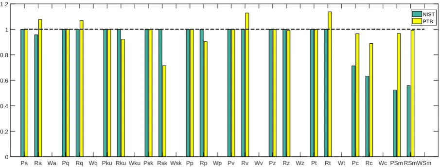
Figure 7. Relative difference graph for theD_coarsetest file, with NPL as the comparison NMI.

NIST shows many parameter values at 1, indicating a good agreement with the NPL value. PTB shows more variation on the roughness parameters.

type F1 reference data files were produced by the University of Huddersfield. This presents the potential for confusion to users, as it would be assumed by many that the datasets would be ready to work with their associated software. Furthermore, of the ten NPL files tested, only two needed any form removal, suggesting the files are not all given in the same condition.

4.6

PTB D_coarse disagreement

One particular file that showed disagreements between PTB and the other two NMIs was the D_coarsefile. The results for this file, with NPL as the comparison NMI, are shown in Figure 7. PTB shows some disagreement forD_coarsein particular for the roughness parameters. The PTB result comes in stark contrast to the relationship between NPL and NIST, which show very good agreement throughout, ignoring the height/spacing parameters. The PTB roughness values do not vary significantly, with the variations being less than 30% of the NPL value, however, the result is interesting when compared to the close agreement that NPL and NIST exhibit.

501E101_4 D_corsEDM16ms EDM Mill SRM3filtered cor10gau impulse lapping01ms millsim

normrand saw123 saw1pad sin1

square steprf stepsrf

0 50 100 150 200 250 300 350 NPL NIST PTB

501E101_4 D_corsEDM16ms

EDM Mill

SRM3filtered cor10gau impulse

lapping01ms millsim

normrand saw123 saw1pad sin1

square steprf stepsrf

0 0.5 1 1.5 2 2.5 3 3.5 4 4.5 5 NPL NIST PTB

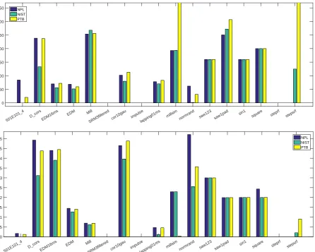
Figure 8. Top: Graph displaying each file result for the RSmparameter. Bottom: Graph

dis-playing each file result for theRcparameter.

NPL and NIST may use the same method.

4.7

Height/spacing parameter disagreements

As was expected, notable amounts of disagreement between NPL, PTB and NIST were found for the height/spacing parameters,XcandXSm. As mentioned above, previous work uncovered some ambiguities in the definition of the RSmparameter that led to the potential for different interpretations to obtain different results [18]. As Xcuses the same discrimination methods as XSm, the same issues are expected to apply. Although Leach and Harris’ work was carried out in 2002, it appears these definitions are still leading to different results. Examples of theXcand XSmresults are shown in Figure 8.

501E101_4 D_corsEDM16ms

EDM Mill

SRM3filtered cor10gau impulse

lapping01ms millsim

normrand saw123 saw1pad sin1

square steprf stepsrf

100 200 300 400 500 600 700 800 NPL_NIST

PTB

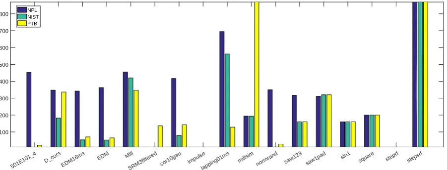
Figure 9. Graph displaying each file result for thePSmparameter.

periodical, simulated test files such assaw1padandsin1, suggesting the software’s tendency to obtain the lower values is related to the methods employed to determine the profile elements, as the very periodic files are more robust to different profile element calculation methods. It ap-pears that the NIST software uses a different interpretation of the height/spacing discrimination definitions, causing it to obtain different profile elements to the other two, and hence different values.

In addition, the PSm results, shown in Figure 9, show NPL obtaining significantly larger values than NIST and PTB for seven data files. Such an effect is not observed on the roughness parameters, suggesting the application of the filter removes this issue. NPL’s tendency to obtain larger values forPSmcould, therefore, be related to the extended length of the profile, as there are no end effects to manage so no ends are cut. The details of the effect are unknown, however, it is likely to be related to the discrimination of the profile elements, as this tendency for larger PSmvalues is not seen for other parameters.

5

Conclusion

differences in the software are varied, and stem from both differing implementations of the same specification standard, as well as potential errors in the coding of the software. In particular, several conclusions can be made:

• The NPL software’s choice of spline interpolation leads to overestimations of sharp steps.

• The NPL software is unable to obtain waviness parameter values for some files, due to omitting profiles with an insufficient number of mean line crossing points per sampling length.

• PTB’s alternative interpretation of waviness profile end management leads to larger wavi-ness parameter values.

• The NIST software fails to obtain values forWcandWSmparameters, potentially due to a misinterpretation of the height discrimination definition.

• Ambiguities in the height/spacing discrimination definitions cause different obtained re-sults for theXSmandXcparameters.

• Lack of guidance in where the sampling lengths should be taken from a profile may lead to different sampling lengths being chosen, and different parameter values being obtained.

• The .SMD file format’s use of control characters leads to a difficulties in use, increasing the likelihood for errors in the file format and reading errors.

The main benefit of this work, through the parameter value differences it has uncovered, is a demonstration of the need for tighter definitions in the specification standards. At present, two reference software packages can give different parameter values for the same file, and thus two different results to compare against. This difference in reference software results can lead to differences in values in collaboration projects involving several companies or institutions, causing disagreements for potentially crucial measurements.

accepts different file formats as inputs. It is suggested that the .SMD file format be removed from ISO 5436-2 and replaced by a more robust format which does not require such specific use of control characters. One potential candidate is the .SDF format, which is already used for areal surface texture, making it familiar to many in the industry, and is much more robust, accepting any combination of <CR> and <LF> to end lines, and ends records simply with a ’*’ [25]. Another possibility is the .X3P format, an open source data format developed by the ’OpenGPS’ consortium [30], currently in use as the default input file-type for the NPL reference software for areal surface texture parameters [31, 32], and defined in ISO 25178-72 [33].

5.1

Further work

Following this research, there is potential for further analysis of the parameter values to uncover the true causes of the currently unexplained discrepancies in the results. Further analysis will require a collaborative effort with the NMIs to delve into the finer details of the software to identify where the different software packages differ on a more specific level.

Additionally, there is potential to begin work on more refined versions of the current ISO def-initions where ambiguities are present. This future work includes the definition of the height/spac-ing discrimination related to the XcandXSmparameters in ISO 4287, as well as the definition of the waviness profile in ISO 4288.

Acknowledgements

We would like to thank the Engineering and Physical Sciences Research Council (EPSRC Grants EP/M008983/1 and EP/1017933/1). Thanks to Dr Peter Harris (NPL) and Dr Dorothee Hueser (PTB) for their valuable comments.

References

[1] A. A. G. Bruzzone, H. L. Costa, P. M. Lonardo, and D. A. Lucca. Advances in engineered surfaces for functional performance.Cirp annals - manufacturing technology, 57(2):750– 769, 2008.

[2] T. R. Thomas. Roughness and function.Surface topography: metrology and properties, 2(1):014001, 2013.

[3] R. Leach.Fundamental principles of engineering nanometrology. Elsevier Science, Bing-hamton, 2nd edition, 2014.

[4] U. Pettersson and S. Jacobson. Influence of surface texture on boundary lubricated sliding contacts.Tribology international, 36(11):857–864, 2003.

[5] P. L. Menezes, Kishore, and S. V. Kailas. Influence of surface texture and roughness parameters on friction and transfer layer formation during sliding of aluminium pin on steel plate.Wear, 267(9-10):1534–1549, 2009.

[6] D. J. Whitehouse.Handbook of surface metrology. CRC Press, 1994.

[7] ISO 16610-21: Geometrical product specifications (GPS) — Filtration — Part 21: Linear profile filters: Gaussian filters. 2011.

[8] ISO 4288: Geometric Product Specification (GPS)— Surface texture— Profile method: Rules and procedures for the assessment of surface texture. 1998.

[9] ISO 4287: Geometrical Product Specifications (GPS)-Surface texture: Profile method–Terms, definitions and surface texture parameters. 1998.

[10] ISO 5436-2: Geometrical product specifications (GPS) - Surface texture: Profile method; Measurement standards - Part 2: Software measurement standards. 2012.

[12] Softgauges for the evaluation of profile suface texture parameters: reference algorithm. URL: http : / / resource . npl . co . uk / softgauges / Ref _ Algo _ Overview . htm (visited on 07/07/2016).

[13] S. H. Bui, T. B. Renegar, T. V. Vorburger, J. Raja, and M. C. Malburg. Internet-based surface metrology algorithm testing system.Wear, 257(12):1213–1218, 2004.

[14] S. H. Bui and T. V. Vorburger. Surface metrology algorithm testing system. Precision engineering, 31(3):218–225, 2007.

[15] Internet based Surface Metrology Algorithm Testing System. URL:http://physics.

nist.gov/VSC/jsp/index.jsp(visited on 07/07/2016).

[16] L. Jung, R. Krüger-Sehm, B. Spranger, and L. Koenders. Reference software for rough-ness analyses - features and results. InXi international colloquium on surfaces. Chemnitz, Germany, 2004, page 164.

[17] RPTB - Software to Analyse Roughness of Profiles. URL:https://www.ptb.de/rptb (visited on 07/07/2016).

[18] R. K. Leach and P. M. Harris. Ambiguities in the definition of spacing parameters for surface-texture characterization.Measurement science and technology, 13(12):1924, 2002.

[19] P. J. Scott. The case of surface texture parameter RSm.Measurement science and tech-nology, 17(3):559–564, 2006.

[20] A. Baker, S. L. Tan, R. Leach, L. Jung, S. Y. Wong, A. Tonmueanwai, K. Naoi, J. Kim, T. B. Renegar, K. P. Chaudhary, O. Kruger, M. Amer, S. Gao, C. L. Tsai, N. Anh, and A. Drijarkara. Final report on apmp.l-k8: international comparison of surface roughness. Metrologia, 50(1A):04003, 2013.

[21] L. Koenders, J. L. Andreasen, L. De Chiffre, L. Jung, and R. Krüger-Sehm. Euromet project 600 - comparison on surface roughness standards. Metrologia, 41(1A):04001, 2004.

[22] T. Li, R. Leach, L. Jung, X. Jiang, and L. Blunt. Comparison of type f2 software mea-surement standards for surface texture.Npl report eng 16, 2009.

[23] I. Paricio, A. Sanz-Lobera, and F. Lozano. Comparative analysis of software measurement standard according to iso 5436-2.Procedia engineering. mesic manufacturing engineer-ing society international conference 2015., 132:864–871, 2015.

[24] ISO DIS 25178-2: 2012 - Geometrical product specifications (GPS) — Surface texture: Areal Part 2: Terms, definitions and surface texture parameters. 2012.

[26] M. Krystek. Form filtering by splines.Measurement, 18(1):9–15, 1996.

[27] ISO 16610-31:2010 - Geometrical product specifications (GPS) - Filtration - Part 31: Robust profile filters: Gaussian regression filters. 2011.

[28] ISO 16610-28: Geometrical product specifications (GPS) — Filtration Part 28: Profile filters: End effects. 2010.

[29] ISO 16610-22:2015 - Geometrical product specifications (GPS) - Filtration - Part 22: Linear profile filters: Spline filters. 2013.

[30] G. Wiora and J. Seewig. Free Interchange of 3D Measuring Data: X3P - a Flexible, System-independent Open Source Data format.Inspect, 11:16–17, 2010.

[31] P. M. Harris, I. M. Smith, R. K. Leach, C. Giusca, X. Jiang, and P. Scott. Software mea-surement standards for areal surface texture parameters: part 1—algorithms. Measure-ment science and technology, 23(10):105008, 2012.

[32] P. M. Harris, I. M. Smith, C. Wang, C. Giusca, and R. K. Leach. Software measurement standards for areal surface texture parameters: part 2—comparison of software. Measure-ment science and technology, 23(10):105009, 2012.

Filter

Parameter Calculation

NPL

SMD file

format Uniformlyspaced removedForm λs filtered

Profile length > 3 cut-off lengths

Points per cut-off length > 50

Gaussian Convolution

Cut-off length removed from

profile Input Data

Piecewise natural cubic spline interpolation

Use Simpson’s rule to obtain estimates of integrations

Evaluate Parameter

Use height discrimination to remove insignificant

profile elements

Am

pl

itu

de

pa

ra

m

et

er

s

Fe

atu

re

pa

ra

m

ete

rs

Output parameters

If primary profile

Figure 10. Algorithm flow diagram for the NPL softgauges software, detailing the routes that

Filter

PTB

PR, SDF, SMD File format

Uniformly spaced

No pre-filtering applied

Input Data

Form-op/ Ls filter order

Ls filter Form operator

16610-21 Gaussian 16610-28 Gaussian

Regression p=1 16610-22 L2 Spline Tilt correction Subtraction of mean None

Lc Filter

16610-21 Gaussian

Fourier 16610-21 GaussianSimple Convolution 16610-28 Gaussian

Regression p=0

16610-22 Spline 16610-28 Gaussian_{Regression p=1} 16610-28 End-weighted Convolution

13565-1 Robust Filter w. Tuckey weighting fn. 16610-31 Gaussian

Regression p=2 16610-31 Gaussian

Regression p=0 (deep pore) 16610-22 L1 Spline

w. 32 V-matrix Ls Value =

None

Lc value = 0.8mm

Form operator and Ls filter can occur in any order (Default 1st_{form, 2}nd_{Ls filter)}

Input Header information

Evaluation length of P Profile

Parameter Calculations

ISO 4287 4.1, 4.2, 4.3: Select parameters to include in

report. for P,R,W

Calculation via summation ISO 4287 4.3 & draft

ISO 21920-2 Annex G: input height 10 & spacing discrim. 1 %

EN 10049 RPc: Input C1

& C2 values (Default = 0.5 and -0.5)

Profile type for material ratio

Method of Abbot algorithm

Height distribution Material ratio

Section height values c_k = height values of profile z_k

If a point has a neighbour below c,

dx/2 is included in hill. Data points sorted

in height order

R,W,P

Create and display Abbot-Firestone

and amplitude distributions Click or type

Mr1, Mr2/ C1, C2 values

ISO 4287: δc

parameter

Rs/R

Create and display Abbot plotfrom ISO 13565-2 defintion

ISO 13565-2: calculate material

ratio parameters

Generate report Use ISO 4287 4.3 or draft

ISO 21920-2 Annex G (Default = both)

End of comparable processes

Figure 11. Algorithm flow diagram for the PTB RPTB software, showing the software route

Filtering

NIST

SMD, SDF, TXT file format

Reference data set Input data

source

Input data set

Curvature removal

Least squares polynomial order 1-20

Best fit polynomial curve fitting (Default order = 1)

Circular fit (under testing)

Filtering method

Gaussian method

2RC method

Fast Gaussian Convolution FFT

Recursive Convolution Gaussian

Window size

0.5 \lambda_c

-0.5 \lambda_c -\lambda_c - \lambda_c Lc value =

0.8mm (Default =

0.08mm)

Require Ls filtering (Default = no)

Ls value (Default =

Parameter Calculations

Surface Parameters

ISO 4287 ASME B46

Height parameters by summation Parameter

choices (Default =

none)

Spacing Parameter sm Spacing 1%

and Height discrim. 10%

(Default 1% and 5%)

Hybrid parameter dq w/ 7 pt. smooth

Calculate uncertainty

Monte Carlo Algorithm % of Pq for

Uz Default = 1%

% of spacing for Ux (Default =

2%

Power Spectral Density

Profile choice

Primary profile

Waviness profile Roughness profile

PSD method

FFT

Mixed Radix FFT FFT zero padding

Windows

Rectangular Hann Hamming Blackman

Caculate (using digitised form) &

display PSD

Auto-Correlation

Profile choice

Primary profile

Waviness profile Roughness profile

Domain choice

Lag Length

Spatial domain Spatial Frequency_domain

Calculate using digitised form

Profile choice

Primary profile

Waviness profile Roughness profile

Domain choice

Lag Length

Spatial domain Spatial Frequency_domain

Calculate using digitised form

2nd_Profile

Bearing area curve

Profile choice

Primary profile

Waviness profile Roughness profile

Calculate & display BAC Number of

bins (Default =

50)

Generate report

Figure 12. Algorithm flow diagram for the NIST SMATS software, showing the software route

NMI Name Type Avg abs Height value (approx. )

# points

NIST Random Roughness Hard coating

Roughness

Specimen <50nm 13197

NIST D_course Roughness

Specimen 2000nm 7998

NPL EDM16ms Master piece 2000nm 22401

NIST EDM Master Piece 300nm 22395

NIST Mill Master Piece 300nm 22395

NIST Bullet Sig 3 SRM 2460 Engraved 250nm&

500nm 5714

NPL Cor10gau Simulated

process 1500nm 5602

NIST Impulse Numerically

Generated 0nm 7998

NPL Lapping01 Master piece 100nm 22401

NPL Mill_sim Simulated

process 500nm 2241

NPL Norm rand Simulated

feature 1000nm 22401

NPL Saw123 Simulated

feature 1000nm 22401

NPL Saw1_pad Simulated

feature 250nm 22401

NPL Sin1 Simulated

feature 500nm 22401

NIST Square Numerically

Generated 1000nm 7998

NPL Step Simulated

feature 500nm 22401

NPL Steps Simulated

feature 0nm 22401

Figure 13. List of files used for testing, taken from the NPL and NIST websites. Each features