High precision lateral distortion correction in coherence scanning interferometry using an arbitrary surface

See discussions, stats, and author profiles for this publication at: https://www.researchgate.net/publication/316428152

High-precision lateral distortion correction in

coherence scanning interferometry using an

arbitrary surface

Conference Paper · April 2017

CITATIONS

0

3 authors, including:

Some of the authors of this publication are also working on these related projects:

EU H2020 ITN MICROMAN “Process Fingerprint for Zero-defect Net-shape MICROMANufacturing” http://www.microman.mek.dtu.dk/View project

Metrology for precision and additive manufacturingView project Richard Leach

University of Nottingham

296PUBLICATIONS 1,774CITATIONS

SEE PROFILE

All content following this page was uploaded by Richard Leach on 24 April 2017.

The user has requested enhancement of the downloaded file. All in-text references underlined in blue are added to the original document

HIGH-PRECISION LATERAL DISTORTION CORRECTION IN

COHERENCE SCANNING INTERFEROMETRY USING AN ARBITRARY

SURFACE

Rong Su

_{, Peter Ekberg}

_{and Richard Leach}

1

_{Manufacturing Metrology Team}

The University of Nottingham

Nottingham, UK

2

_{Department of Production Engineering}

KTH Royal Institute of Technology

Stockhkolm, Sweden

INTRODUCTION

Lateral optical distortion is present in most optical imaging systems. In coherence scanning interferometry (CSI) [1,2], distortion may cause field-dependent systematic errors in the measurement of surface topography. Distortion, unlike optical aberrations such as spherical aberration, coma and astigmatism, is not responsible for a lack of sharpness of the image [3]; rather is related to the form of the image, and the degree of the distortion is dependent on the position in the image plane. Optical aberrations are usually suppressed for optimisation of the optical resolution in a commercial CSI system, but a significant amount of distortion can be present [4,5]. In areas such as computer vision, distortion in a camera system may cause errors in pattern analysis and recognition, dimensional and displacement measurement, 3D image reconstruction, etc. [6]. In a CSI system that measures the 3D topography of a surface, distortion may cause errors in the dimensional measurement in both lateral and height directions. Thus, distortion should be corrected in order to achieve a non-distorted image field and a uniform lateral sampling distance of the image projected on to the camera, such that the measurement accuracy can be improved.

Two steps are usually required to correct lateral distortion: 1) correct the form of the image, e.g. when imaging a perfect grid pattern the systematic deformation of this grid should be removed so that the measured grid has uniformly distributed nodes; 2) absolute calibration and adjustment of the scale, i.e. the scale of the image should be made traceable to the definition of metre (a linear scaling problem).

The traditional calibration and adjustment of the lateral distortion for a 3D imaging system

combines the two steps listed above into one by measuring a standard artefact. The artefact usually contains a grid of precision manufactured patterns, mostly with rectangular or circular shapes, e.g. an areal cross grating standard [7]. The distortion is then calculated as the deviation of the measured positions of the patterns compared to their nominal positions. The nominal positions are calibrated by a traceable metrological instrument, e.g. a stylus instrument [8]. The manufacturing and calibration processes of the standard artefact are often complex and expensive.

Self-calibration techniques may also be used for distortion correction [4,5]. When using self-calibration techniques, the distortion correction may be separated to the two steps mentioned above. However, current self-calibration methods still require an artefact with a grid of manufactured patterns. After the separation of the distortion and the shape error of the artefact, the absolute scale may be determined using a linear scale artefact that is traceable to metre.

systems with different lenses and magnifications, a range of grids with suitable pitches is required.

In this paper, a new method for the correction of lateral distortion in a CSI system, based on a simple sub-pixel imaging correlation method and self-calibration, will be demonstrated. Instead of using a manufactured grid pattern, an arbitrary surface is used and a precision of a few nanometres is achieved for the distortion correction. Here, an arbitrary surface refers to a surface that contains some deviations from flat and has some features (possibly just contamination), such that feature detection is possible. This surface could be a rough surface, e.g. a regular machined metal surface or the surface of a coin, or it could be a smooth surface with random features or structured patterns, e.g. a scratched and defected mirror or an areal cross grating. These surfaces can be easily found in a laboratory, manufacturing workshop and even an office. The method demonstrated in this paper may significantly enhance the precision of the distortion correction of 3D optical imaging systems. The cost of the artefact may be reduced significantly and even to zero if the absolute scale is not considered.

METHODS

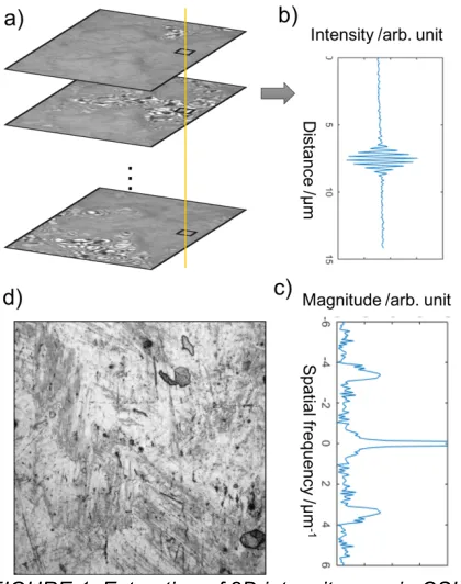
Extraction of 2D intensity map in CSI

In CSI, the height variation is encoded into the phase of the complex wave amplitude [1,2]. The low spatial frequency term of the CSI signal corresponds to the intensity signal without interference effects and can be extracted by

using low-pass filtering (see FIGURE 1). The

extracted two-dimensional (2D) intensity map will be used for further analysis. The CSI instrument used in this study has a precision piezo-electric drive with a maximum scan speed of 96 μm/s. The specifications of the objective lens used in this study are given in Table 1.

TABLE 1. Specifications of the objective lens

Magnification Type NA

50× Mirau 0.55

Field of view (FOV) /µm

Optical resolution

/µm

Lateral sampling distance /µm

166.912 0.52 0.163

FIGURE 1. Extraction of 2D intensity map in CSI. a) Interferometirc image stack in CSI; b) interference signal recorded by a pixel; c) the Fourier transform of the signal, where the low frequency part corresponds to the intensity map; d) the extracted intensity map.

Image correlation method

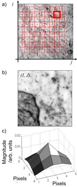
Image correlation methods have been widely applied in many areas, such as the measurement of stress, strain and displacement in the field of mechanics [9]. In this study, the first step of the image correlation method is the definition of the grid of image patches in the 2D intensity map extracted from the measured CSI data of a surface. Usually measurements from three different views are required for a self-calibration process [10]. The first view is called the reference view, based on which the grid is defined (see FIGURE 2). The translated and rotated views are defined as the measurements of the same area of the surface but being slightly shifted and

approximately 90° rotated, respectively. The

defined grid on the arbitrary surface is equivalent to the physical grid manufactured in a standard artefact. One of the advantages is that the location and pitch of the defined grid is known and may be easiliy adjusted so that any spatial frequency of the distortion can be captured.

Searching for the exact positions of the image

patches (e.g. see FIGURE 2(b)) in the translated

the cross correlation function between two image patches; one from the reference view and the other from the translated or rotated view. This process does not require high precision and is carried out by using a priori information of the translation and rotation, i.e. the translated distance and the degree of the rotation angle. The cross correlation function can be expressed as

𝐶",$ 𝑝, 𝑞 = 𝑓 𝑖 − 𝐼, 𝑗 − 𝐽 .

𝑔 𝑖 − 𝐼 + 𝑝, 𝑗 − 𝐽

1

+ 𝑞 ,

where 𝐼, 𝐽 is the centroid position of an image

patch in the reference view in the image

coordinate system 𝑖, 𝑗 , which corresponds to the

x and y directions in the spatial domain,

respectively. Functions 𝑓 𝑖, 𝑗 and 𝑔 𝑖, 𝑗 are the

intensity maps of the image patches in the reference view and the translated or rotated view, respectively. Because the images of all three views are aligned using a priori knowledge of the translation and rotation, the searching area can

be as small as a few pixels around 𝐼, 𝐽 . The pixel

coordinates 𝑝, 𝑞 , corresponding to the

correlation maximum, are the desired quantities.

The entire set of 𝑝, 𝑞 for all image patches

provides the location of the defined grid with pixel-precision in the translated or rotated view.

The result of the correlation function is refined with sub-pixel precision, which can be achieved by resampling the image patches using a cubic interpolation combined with a simple iterative method for searching for the correlation maxima. In principle, the grids calculated from the repeated measurements of the reference view should overlay the defined grid, and the grids calculated from the other views should appear distorted.

2D self calibration method

Reversal techniques and other forms of self-calibration have been used for centuries in order to calibrate machine tools and metrology instruments [10]. The mathematical theory behind the 2D self-calibration technique in metrology systems was developed by Raugh [11]. A numerical approach for solving the self-calibration problem, based around the concept of iteration, was developed by Ekberg et. al. [12]. In

general, 2D self-calibration is based on the

assumption that the artefact will not change its shape regardless of how it is mounted in the measuring instrument, i.e. it is a rigid body. Then the apperant shape of the artefact will change when it is observed at different positions in the

measuring instrument, if lateral distortion is present. It is possible to separate the distortion and the real shape of the artefact, by using at least three measurements of the same artefact with different placements. The typical placement scheme contains a reference measurement, a translated measurement and a measurement with the artefact rotated. The details of the 2D self-calibration method can be found elsewhere [12].

FIGURE 2. Illustration of the image correlation method. a) A 9-by-9 grid of image patches defined in the 2D intensity map of the CSI measurement of a coin surface; b) the enlarged image patch (100-by-100 pixels) of which the centroid is located at 𝐼, 𝐽 in the image coordinate; c) the correlation function which is the result of searching for the reference image patch around 𝐼, 𝐽 in the translated or rotated views.

RESULTS

coin surface, and the image patches are defined based on the intensity map of a single reference

measurement. The height information in FIGURE

3(c) is used for the estimation of the best focus

position along the scanning axis.

FIGURE 3. Extraction of the 2D intensity maps from CSI measurements of a coin surface and definition of the grid. a) Picture of the coin; b) an image slice from the 3D fringe data; c) calculated height map; d,e,f) Intensity maps of the reference, translated and rotated views, respectively; g) defined grid and image patches. The grey scales of all intensity images are normalised. The 50× objective lens was used.

The nominal grid is defined as a perfect square area containing 9-by-9 image patches as shown in FIGURE 3(g). The centroids of the image patches are calculated using the described image correlation method, such that the grid can be

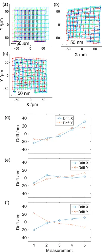
presented by 9-by-9 nodes. FIGURE 4 shows the

grids that are calculated from the repeated measurements of the three different views. The measured grids from the translated and rotated

views are distorted because of the presence of optical distortion. This procedure is repeated five times to evaluate the measurement repeatability and overlay of the instrument. The overlay is the limiting factor of the precision of the self-calibration method, and is calculated as the standard deviation of the distances between the measured positions of the nodes (centroids of the image patches) and the corresponding mean position calculated from the five measurements.

The measured grids are shown in FIGURE 4(a)

to FIGURE 4(c). It should be noted that the repeated measurements are not overlapping perfectly, which indicates possible lateral drifts of

the image domains of the repeated

measurements. The drift can be evaluated as the relative offsets of the centroids of the grids (see FIGURE 4(d) to FIGURE 4(f)).

The measured grids can be aligned with their centroids for all the nodes in order to calculate the measurement overlays. The calculated overlay is around 1 nm for all three views. The overlay is mainly associated with the measurement noise that is influenced by environmental changes, vibration, electronic noise, etc. [13].

The drift is of the order of tens of nanometres and is probably caused by the motion of the axial scanner. The drift of the entire image domain can hardly be noticed in a scanning-type microscopic imaging system where the lateral sampling distance in an image is usually in the range from 100 nm to 6 µm. The drift may degrade the repeatability of the instrument.

The input to the self-calibration algorithm is the measured grids from the three different views, as

shown in FIGURE 5(a) (aligned with the centroids

for display purposes). The output is the distortion

map (FIGURE 5(b)), from which the distortion

function and the correction function can be obtained. By applying the correction function to the three measurements, the distortions in the translated and rotated views can be corrected

(see FIGURE 5(c)). Due to the system noise, the

lens with much lower magnification (to be reported in a later publication).

FIGURE 4. Measured grids from three different views. a,b,c) Resulting grids (absolute coordinates) of the repeated measurements of the reference, translated and rotated views, respectively (the errors are magnified for visualisation purpose); d,e,f) calculated drifts for the reference, translated and rotated views, respectively.

FIGURE 5. Self-calibration result. a) Input to the self-calibration algorithm and the placement scheme; b) calculated distortion of the CSI system with 50× magnification lens; c) overlay of the distortion-corrected grids.

TABLE 2. Measured distortion and evaluation

x y

Distortion /nm

Maximum

value 72 50

RMS residual errors /nm

Reference

view 2 2.2

Translated

view 2.4 2.1

Rotated

view 2.4 2.2

CONCLUSION

with structured patterns, the new approach makes use of an arbitrary surface that can be easily found, e.g. a coin surface. A precision of a few nanometres can be achieved for the distortion correction over a large FOV. The spatial sampling of the distortion is no longer limited by the structures in the artefact. A rarely observed drift due to the axial scanner in CSI has also been found, and the drift is of the order of a few tens of

nanometres. Although an absolute scale is still

needed to make the calibration traceable, the problem of obtaining the traceability is simplified as only an accurate measure of the distance between two arbitrary points is needed. Thus, the total cost of transferring the traceability may be reduced significantly using the new approach. In the future, a new method that may simplify the way of obtaining absolute scale will be investigated, and a 2.5D self-calibration method will be developed for correction of field curvature effect in CSI.

ACKNOWLEDGEMENTS

This work was supported by the Engineering and Physical Sciences Research Council (EPSRC) (EP/M008983/1).

REFERENCES

[1] de Groot P, Principles of Interference Microscopy for The Measurement of Surface Topography, Advances Optics and Photonics. 2015; 7: 1-65.

[2] de Groot P, Chapter 9. Coherence Scanning Interferometry, in Optical Measurement of

Surface Topography, 
Leach R K, ed.

Springer, Berlin Heidelberg, 2011. 


[3] Born M, Wolf E. Principles of Optics: Electromagnetic Theory of Propagation, Interference and Diffraction of Light, Cambridge University, Cambridge: 1999. [4] Henning A, Giusca C, Forbes A, Smith I,

Leach R K, Coupland J M, Mandal R.

Correction for Lateral Distortion in

Coherence Scanning Interferometry, CIRP Annals – Manufacturing Technology. 2013; 62: 547-550.

[5] Ekberg P, Mattsson L. A New 2D Self-Calibration Method with Large Freedom and High-Precision Performance for Imaging Metrology Devices, Proceedings of the 15th International Conference of the European Society for Precision Engineering and Nanotechnology, Elsevier, 2015, 159-160. [6] Yoneyama S, Kikuta H, Kitagawa A,

Kitamura K. Lens Distortion Correction for Digital Image Correlation by Measuring

Rigid Body Displacement, Optical

Engineering. 2006; 45: 023602.

[7] Leach R, Giusca C, Cox D, Guttmann M, Jakobs P-J, Rubert P. Development of Low-Cost Material Measures for Calibration of the Metrological Characteristics of Surface Topography Instruments, CIRP Annals – Manufacturing Technology. 2014; 64: 545-548.

[8] Leach R K, Giusca C, Naoi K. Development and Characterization of a New Instrument for the Traceable Measurement of Areal Surface Texture. Measurement Science and Technology. 2009; 20: 125102.

[9] Sutton M, Orteu J, Schreier H. Image Correlation for Shape, Motion and

Deformation Measurements: Basic

Concepts, Theory and Applications.

Springer, US, 2009.

[10] Evans C, Hocken R, Estler W, Self-Calibration: Reversal, Redundancy, Error Separation, and ‘Absolute Testing’, CIRP Annals – Manufacturing Technology. 1996; 45: 617-634.

[11] Raugh M, Absolute Two-Dimensional Sub-Micron Metrology for Electron Beam Lithography – A Calibration Theory With Applications, Precision Engineering. 1985; 7: 1-13.

[12] Ekberg P, Stiblert L, Mattsson L, A New General Approach for Solving The Self-Calibration Problem on Large Area 2D Ultra-Precision Coordinate Measurement Machines, Measurement Science and Technology. 2014; 25: 055001.

[13] Giusca C, Leach R K, Helary F, Gutauskas T and Nimishakavi L. Calibration of the Scales Of Areal Surface

Topography-Measuring Instruments: Part 1.

Measurement Noise and Residual Flatness. Measurement Science and Technology. 2012; 23: 035008.