A case of framing effects : the elicitation of time preferences

S

c

h

o

o

l

o

f

E

c

o

n

o

m

ic

s

&

F

in

a

n

c

e

D

is

c

u

s

s

io

n

P

a

p

e

r

s

A Case of Framing Effects: The

Elicitation of Time Preferences

Paola Manzini and Marco Mariotti

A Case of Framing Effects: The Elicitation of Time

Preferences

Paola Manzini

University of St. Andrews and IZA

Marco Mariotti

Luigi Mittone

Abstract

We compare three methods for the elicitation of time preferences in an experi-mental setting: the Becker-DeGroot-Marschak procedure (BDM); the second price auction; and the multiple price list format. The first two methods have been used rarely to elicit time preferences. All methods used are perfectly equivalent from a decision theoretic point of view, and they should induce the same ‘truthful’ rev-elation i dominant strategies. In spite of this, we find that framing does matter: the money discount rates elicited with the multiple price list tend to be higher than those elicited with the other two methods. In addition, our results shed some light on attitudes towards time, and they permit a broad classification of subjects depending on how the size of the elicited values varies with the time horizon.

J.E.L. codes: C91, D9

Keywords: time preferences, elicitation methods, BDM, Auctions, MPL

∗_{We wish to thank all the tireless staff at CEEL, and in particular Marco Tecilla, for the excellent}

1

Introduction

Many experimental studies elicit preference parameters (such as risk aversion or discount rates) from subjects. In economics experiments, a major preoccupation is that of making the elicitation incentive compatible: the ‘true’ response should be the dominant response for the subject among the available ones, whatever her true parameter happens to be. Often, for a given parameter to be elicited, there exists several elicitation mechanisms that are both a priori appealing and incentive compatible, and that thus should theoret-ically yield the same (true) response from subjects. In this study, we compare three such theoretically equivalent incentive compatible methods for the elicitation of time prefer-ences and test whether the theoretical equivalence is confirmed in the laboratory. In an experimental setting we can control other factors influencing subjects’ choices: thus any observed discrepancy can only mean that factors intrinsic to way choices are presented to the subject, and which should be irrelevant for the agent’s response, do in fact matter. For this reason we call such factors framing effects. Our main conclusion will be that there is evidence of framing effects in subjects’ responses. Nevertheless we also obtain some frame independent results that may be of interest.

A first reason for focussing on time preferences is simply the obvious importance of the topic. Many economic decisions have a crucial time dimension (e.g. investments, pensions) and therefore it is important to develop accurate theoretical models and reliable empirical methods to elicit the time preferences of individuals. A second reason is that eliciting time preferences has proven to be far from a trivial matter. For example, one of the more puzzling findings is the wide variety of ranges for discount factors estimates (see e.g. Table 1 in Frederick, Loewenstein and O’Donoghue [13]); and even within a single class of preference elicitation method, results are sensitive to the details of the experimental design (see e.g. Dohmen, Falk, Huffman and Sunde[11]). Thirdly, studies in this vast literature do not proceed in a standard way, and many are the confounding factors from one study to another, which hamper systematic comparisons to determine to what extent these differences depend on the elicitation methods themselves as opposed to other differences in experimental design. In a nutshell, at the level of experimental design the main issues that emerge are the following:

• not all studies elicit time preferences in an incentive compatible way;

from serious incentive properties in the neighbourhood of the truth telling dominant strategy: Deviations may be ‘cheap’ enough that experimental subjects do not select the dominant strategy;1

• the above aside, some recent theoretical advances even put into serious question the conventional interpretation of established empirical evidence.2

In this paper we compare three methods to elicit time preferences. For all of them, we focus on eliciting the maximum amount subjects are prepared to pay in order to anticipate receipt of a monetary reward (“speed-up” condition). We investigate whether or not the various elicitation procedures yield consistently different results. The methods we consider are widely used as general elicitation techniques, though not in all cases for time time preferences. The first is the Multiple Price List Method (henceforth MPL), currently the most used technique for preference elicitation in the time domain. In addition, the so called Becker-DeGroot-Marschak [5] (henceforth BDM) and the ‘second price sealed bid auction’ (henceforth ‘Auction’) are the most widely relied upon methods to elicit ‘home-grown’ values in the goods domain. As far as we are aware, the BDM has been used in the time domain only twice before,3

and in a paper and pencil settings as opposed to computerised sessions. Auctions too have been used very rarely in the past for the elicitation of time preferences, and anyhow prevalently in the psychology rather than the economics literature.4

1

See Harrison, Lau and Rutstrom [18] for other common elicitation pitfalls.

2

For instance Noor [29] and Halevi [14] are recent papers challenging the conventional wisdom re-garding hyperbolic discounting. Noor [29] starts from the observation that evidence of high impatience toward immediate rewards is compatible not just with hyperbolic discounting, but also with experimen-tal subjects being likely to be cash constrained; he performs a calibration exercise and shows that the evidence is compatible with standard exponential discounting under certain additional condition. Halevi [14] studies the relationship between time inconsistency and stationarity of time preferences, challenging the current view that time inconsistent choices arise mainly from present biased preferences, since in his

study he finds that half of the subjects with timeinconsistent choices exhibit stationary time preferences

(and one third of the subjects who are time consistent exhibit non stationary choices). More in general, Cubitt and Read [10] discuss the problems when eliciting discount factors in the lab.

3

See Manzini [25] and Benhabib, Bisin and Schotter [6].

4

See e.g. Kirby and Marakovich [21], who compare real and hypothetical delayed rewards within a

first price auction mechanism, in rather small samples (22 subjects in the real reward treatment, and 20 in the hypotehtical treatment). Kirby [20] uses a second price sealed bid auction. Here, though, subjects had to use their own money to bid to have the right to receive a delayed reward (i.e. the question asked

was “The item up for auction is $X. The most I would be willing to pay for this item immediately is ...”,

More in general, papers comparing different elicitation methods for time preferences are very few5

- yet in different domains, most notably in the pricing of goods, various alternative methods have been employed.6

The Multiple Price List method falls into the category of choice tasks: subjects are simply asked to choose between two different amounts available at different dates. The other two methods, Auction and BDM are matching tasks: broadly speaking, subjects have to specify what amount available earlier would be equivalent to a later, fixed reward. That pricing and matching tasks can give rise to different evaluations has been known for a long time, but in situations not involving delayed rewards.7

In the time domain, Read and Roelofsma [36] study whether differences might emerge, and although they do find some evidence for this (i.e. their subjects are less patient when answering choice rather than matching questions), their experiment was conducted using hypothetical payments, and the choice task did not use an incentive compatible mechanism.8

In our experiment the elicitation methods are incentive compatible: declaring one’s true time preference’ is a weakly dominant strategy. Furthermore, as described in detail in section 3, in our implementation these three elicitation methods arestrategically

equiv-alent: from a standard decision theoretic point of view there is absolutely no difference

between them. The only differences are in the ways the problems are framed, and a de-cision maker that ignores irrelevant features beside economic incentives should make the same choices in all of them.

Contrary to this benchmark expectation, we find that the methods do differ. First of all, money discount factors elicited with the MPL method are smaller than those elicited

experimental design is close in spirit to Horowitz [19], where subjects bid for bonds that matured with delay. In our own experimental design the objective is to elicit the bid that makes the subject indifferent between receiving a larger sum later (LL) or the (elicited) smaller reward sooner (SS). That is, we believe that our experimental design makes immediately clear what SS and LL are.

5

Hardisty et al. [15] compare choice (as in the MPL) and matching (as in BDM and Auctions) methods for the elicitation of time preferences in mostly hypothetical choices, and do find differences in the results obtained.

6

See e.g. Shogren et. al [38] and Noussair et al. [30] for comparisons of auction methods and BDM.

7

The first paper to uncover such differences is Lichtenstein and Slovic [23].

8

under the two other frames. Secondly, unlike previous evidence in domains different from time,9

we find that the BDM and the Auction method provide similar elicited values (with some caveats). Finally, looking at individual responses we find that subjects can be classed into three groups, broadly corresponding to increasing, decreasing and non monotonic time preference profiles, depending on how the size of the elicited values varies with the time horizon.10

The rest of the paper is organised as follows. We explain the elicitation methods used in the next section, where we also describe our experimental design. We discuss the strategic equivalence between the three elicitation methods used in section 3. The results are reported in section 4, with further details confined to the Appendix, which also includes the experimental instructions. Section 5 concludes.

2

Experimental design

We ran four session for each of the three treatments (MPL, BDM, second price Auctions), with 16 subjects per session - of the 20 initial participants in each session only the fastest 16 who answered correctly a simple comprehension test (administered after reading the instructions) continued to the experiment proper (the others were given the show up fee and left).11

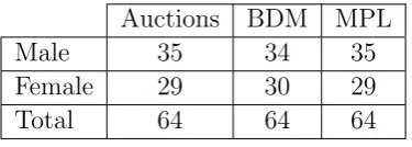
Auctions BDM MPL Male 35 34 35 Female 29 30 29 Total 64 64 64

Table 1: The treatments

We elicited the willingness to pay to anticipate to the following day the receipt of a e_{20 otherwise available with three different delays, of 1, 2 and 4 months (as in e.g.}

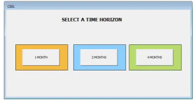
Harrison, Lau and Williams [17]), using an ’overlapping design’ framework, in the sense that all time horizons are compared with the same origin.12

We implemented this by

9

See e.g. Rutstr¨om [37] or more recently Noussair, Robin and Ruffieux [30].

10

For recent evidence on negative time discounting in an experiment with hypothetical questions see Casari and Dragone [8].

11

In spite of this element outside our control, treatments remained evenly balanced in terms of the sex of the participants.

12

presenting subjects with a screen with three buttons, each corresponding to one of the time horizons.

Figure 1: Selecting a version

After completing each choice task, subjects were sent back to this screen with the button corresponding to the time horizon already “played” appearing greyed out. In addition to a fixed participation fee, 50% of the subjects in each group were drawn at random to receive a payment consistent with their choices (we explain more precisely how for each of the three methods below): at the end of the experiment we drew from a uniform distribution which 8 subjects (out of 16 participants in each computerised session) would receive a payment in addition to the show up fee; which screen (1 month, 2 months or 4 month delay) would ’count’, and, in the case of the MPL elicitation method, which row in that screen (the payment corresponding to the option, A or B, chosen in that row) would be selected for payment.

Subjects could enter money amounts in 50 eurocents increments. This has the advan-tage of making possible mistakes more costly for subjects (see Harrison [16]), and since we are not interested in the estimation of discount factors but only in the comparison of alternative elicitation methods, having a coarse grid of elicited values is not an issue. We have followed the current practice (see e.g. Filiz-Ozbay et al. [31]) not to indicate the interest rates corresponding to each choice.13

Nevertheless, in the second part of the

months, 6 to 12 months) designs, and show that different designs do have an effect on the elicited values. Though we use the overlapping design, we do this for all treatments, so that any differences we find do not have to do with the specific design. An open question is whether a shift design would produce different results.

13

experiment we test the subject awareness of the interest rates implied by their choices, in order to obtain an approximate measure of how relevant these rates were for making the decision. After all values have been elicited, subjects are asked to state the three interest rates corresponding to their choices and referred to the specific time horizon. So, for instance, a declaration of e_{18 in the two month horizon question would have an}

im-plied rate of 10% for the month, with no need to report the interest imim-plied on an annual basis. These questions were incentivised, being remunerated at e_{2 or} e_{1 depending on}

whether the answer was within a 5% or 10% margin, respectively, of the true rate. Of course the ability to provide a correct answer relies on memory, computational ability and attention - we are not trying to test which of these aspects is more relevant. Only 17%, 12% and 9.8% come within 10% of the correct rate for one, two and four months horizon, respectively. We report a full analysis of these errors in section 4 together with our other results. Finally, we administered a simple questionnaire to elicit information on personality traits, which we use mostly to verify the balancedness of our samples across treatments in terms of these characteristics.

In summary, then, our experiment consisted of five phases for each of our three treat-ments: 1) general instruction, 2) incentivised comprehension test (only the quickest 16 providing correct answers would continue to the next phase), 3) incentivised elicitation of money discount factors (over three time horizons), 4) incentivised elicitation of perceived interest rates (corresponding to the choices in the three time horizons), 5) HEXACO questionnaire on personal characteristics.

2.1

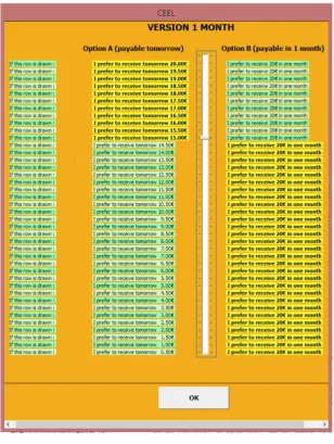
MPL

We implemented the MPL elicitation method with a single switching point:14

the subject is in essence asked to state the (minimum) value he is prepared to accept to avoid waiting for the full amount L later. In other words, he prefers to receive any amount equal or

getting, it is pretty clear to us that their level of financial competence when it comes to interest rates is

less than expert (!). As for savings accounts, in the pilot about a third of subjects - 118 - declared they

had one. Of these, 49, i.e. around 40%, stated they knew what the interest rate they were getting was, but 14 of these – i.e. almost 30% - stated a rate of at most 1%, and a further 16 stated rates between 1 and 2%: if this is really what they were getting, it was not a good deal!

14

greater to the switching value s at an earlier date rather than receive L later. A sample screenshot is reported in figure 2. Truth telling is a (weakly) dominant strategy (and arguably the MPL elicitation method makes the optimality of truthtelling much easier for participants to realise15

as compared to alternative methods). Appendix B explains this point in detail for all three elicitation methods.

Figure 2: Sample Screenshot for MPL elicitation method

15

2.2

Auctions

We implemented a sealed-bid second-price auction to make it as similar as possible to the setups in the other two elicitation methods. When auctioning a good, it is pretty clear to participants that what they are offering is a price to obtain the good. In our case the good in question is time: so subjects were asked to state the minimum amount they were prepared to accept in order to anticipate receipt. This is arguably a direct way to frame the problem which is easier for participants to understand, as compared to asking them to state how much they would be prepared to pay in order to anticipate receipt, and then work out by themselves how much money they would actually receive. The participant stating the lowest amount would ‘win’ the auction and, if drawn, receive an amount equal to the second lowest bid on the following day. A ‘loser’ would receive, if drawn, the full amount with delay. A sample screenshot is visualised in figure 3.

Figure 3: Sample screenshot with the elicitation question for the auction method

2.3

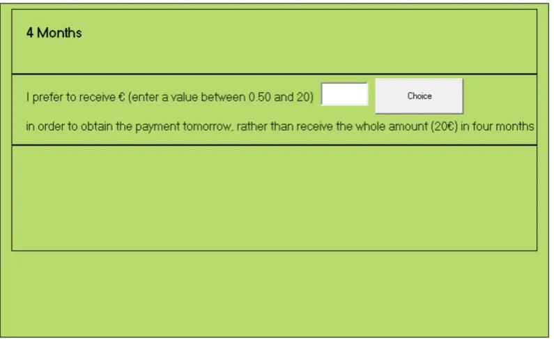
Becker-DeGroot-Marshack (BDM)

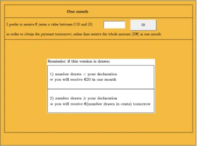
As in the Auction treatment, in our implementation of the BDM mechanism subjects were are asked to state the minimum amount they would be prepared to accept in order to anticipate receipt instead of waiting to receive the whole amount with delay. For each of the three time horizons, if the value declared was not larger than a value drawn from a uniform distribution with support up to L, then the subject would receive a payment equal to the number drawn the following day. Otherwise he would get the full amountL with delay. A sample screenshot is in figure 4.

Figure 4: Sample screenshot for the BDM elicitation method, two month version

3

Strategic equivalence

as well as the values declared in the Auction and BDM methods. We use the term ‘value drawn’ to refer to the second highest declared value in the Auction method and the value of Option A in the row drawn in the MPL method, as well as the value drawn in the BDM method. The ‘small sooner’ amounts are paid with a delay of one day - nevertheless in what follows we refer to ‘immediate’ payment or to payment ‘without delay’ to distinguish it from the case when the payment is delayed by one, two or four months.

For all three methods the grid of available declarations was from e_{0.50 to} e_{20.00 in} e_{0.50 increments; in all elicitation methods:}

• the declaration determines whether payment is anticipated or not: it is anticipated if the value drawn (row drawn for tables, number drawn for BDM, second lowest bid for Auction) is higher than or equal to the declaration (smallest value of option A for tables, number declared in Auction and BDM), and it is delayed if the value drawn is smaller than the declaration.

• a declaration of e_{0.50 ensures the payment will not be delayed, though the payoff}

may be as low as e_{0.50 (if such low value were drawn);}

• a declaration ofe_{20 ensures that the full payment will be received at the later date,}

and with probability 1/40 (i.e. ife_{20 were drawn) the full amount could be received}

without delay;

Next, we show that in each elicitation method declaring the true value is a weakly dom-inant action, and establish the strategic equivalence of the three methods by displaying a one-to-one correspondence between the strategy spaces and the payoffs of each of them with those of the others.

The strategy space for agent iin methodm ={M, B, A}(for MPL, BDM and second price Auctions, respectively) is Sm

i = {0.50,1, ...20} for all m. Let N denote ‘Nature’,

i.e. the random draw, which ‘plays’ in the BDM and Tables method, and let d denote the value drawn. Assume rational agents with standard time preferences, so that for each of them there exists a unique value s⇤

i such that (s⇤i,0) ⇠i (20,1). The payoff to agent i

playing in treatmentm is

πB(si, d) =

⇢

(d,0) if si d

(20,1) ifsi > d

πM(si, d) =

⇢

(d,0) if si d

(20,1) ifsi > d

πA(si, s−i) =

⇢

(d,0) if si d= min{sj :j 6=i}

so that the best reply correspondenceBm in treatment i is given by

BB(d) = 8 < :

{si :si d} if s⇤i < d

{si :si d} if s⇤i =d

{si :si > d} if s⇤i > d

=BM(d) =BA(s₋i)

where as before in the case of auctions d= min{sj :j 6=i}.

4

Results

The bulk of our analysis revolves around what we term ’money discount factors’, calculated simply by dividing the declared values s(smaller sooner) by the total delayed amount L, that is as s

L100.

16

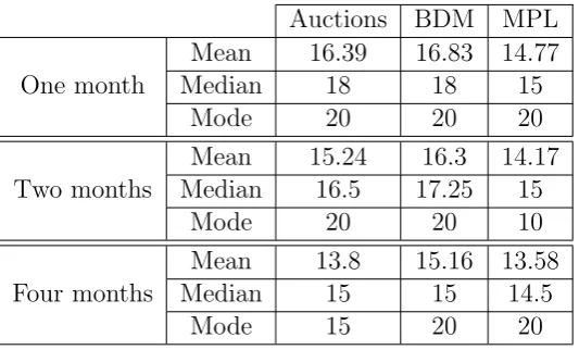
As already anticipated, we find that the methods do differ in terms of elicited values (see Table 3). We can summarise our results as follows:

1. if we look at aggregate data, the three methods generate broadly different median and mean money discount factors (Table 2): across treatments, the mean elicited values are smallest for MPL and largest for BDM, with Auctions ‘in the middle’; similarly for median elicited values, where however these coincide for MPL and BDM for the two months and four months horizons. Broadly speaking, these differences are statistically significant.

2. if we look at individual data, we see that in each treatment subjects can be classed into three distinct groups, based on the values that they declare for each of the three time horizons (Table 4). One group consists of subjects who declare (weakly) smaller values as the time delay increases, in line with the standard exponential discounting model. We call these subjects ‘Time is Money’ (TIM). A second group displays the exactly opposite behaviour, declaring values that (weakly) increase as the time to receipt of the full payment increases (TIP subjects, for ‘Time Is Plea-sure’). A third group has non-monotonic declarations, with either a ‘hump’ or a

16

The unit of measurement of 50 eurocents is also the inbuilt margin of error in the elicitation of the

true value. That is, we can assume that any amount elicited through these methods was within 0.5e_of

the ‘true’ values∗_{, which would lie within the range [s−0.50, s]. Computing the money discount factors}

as the ratios between the elicited values and the total amounts changes the range to⇥s₋0.5

L 100, s L100

⇤

,

which 2.5% wide. Since the incentives are for subjects to state the highest possible values that they are

Auctions BDM MPL Mean 16.39 16.83 14.77 One month Median 18 18 15

Mode 20 20 20 Mean 15.24 16.3 14.17 Two months Median 16.5 17.25 15

Mode 20 20 10 Mean 13.8 15.16 13.58 Four months Median 15 15 14.5

Mode 15 20 20

Table 2: Elicited values by treatment

‘bowl’ shape (henceforth HUBO), that is declared values that are either highest or lowest for the two months horizon as compared to the one and four month horizons. In addition, controlling for these time preference profiles, it emerges that the differ-ences in elicited values across methods are driven mainly by the declarations of the arguably more rational agents, the TIMs.

3. Subject whose declarations decrease with the time horizon (the ‘more rational’ sub-jects) also appear to make fewer errors: when asked about the internal rate of return corresponding to their choices, a larger proportion of TIMs assesses correctly the discount rate corresponding to their declaration as compared to subjects with dif-ferent time preference profiles. In addition, mistakes are smaller in absolute value. Finally, TIP subjects tend to overestimate their errors as compared to TIMs

The rest of the section is devoted to analysing these results.

4.1

Time preference profiles and elicited money discount rates

We begin by reporting the descriptive statistics of the declared values in the three treat-ments:

In addition, we report below the whole distributions of the elicited values by elicitation method.

Figure 5: Distribution of elicited values by treatment

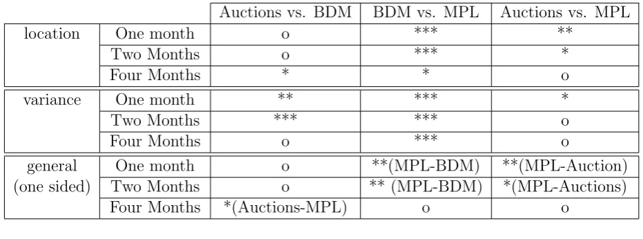
central location, assuming that the two distributions being compared have the same vari-ance; Conover test to detect differences in variance between two distributions that does not assume equality of either location or scale; and two sample Kolmogorov-Smirnov test (henceforth KS), which is an omnibus test for the equality of two distributions against the alternative that they are different (in either scale or location). The one sided KS test detects when one distribution obtained with elicitation method X stochastically domi-nates another distribution obtained with elicitation method Y. Thus we say that X-Y is statistically significant as a shorthand for the observation that method X elicits values which are consistently smaller than those elicited by method Y.

We find that the differences reported in Table 2 and Figure 5 are statistically significant if we compare the MPL with any of the other two elicitation methods, the only exception being the difference between Auctions and MPL in the four month horizon. Whenever the differences are statistically significant, both Auctions and BDM elicit consistently lower declarations than the MPL method (see Tables 15 and 14in the Appendix), with the distribution of values elicited in the MPL method dominated stochastically by those with both of the other methods.

Auctions vs. BDM BDM vs. MPL Auctions vs. MPL

location One month o *** **

Two Months o *** *

Four Months * * o

variance One month ** *** *

Two Months *** *** o

Four Months o *** o

general One month o **(MPL-BDM) **(MPL-Auction) (one sided) Two Months o ** (MPL-BDM) *(MPL-Auctions)

Four Months *(Auctions-MPL) o o

Legend (significance value) ***: 1%, **: 5%, *: 10%,

o: statistics p-value is greater than 10%

Table 3: Summary of differences between distributions of elicited values

the same variance. However for more general differences in distributions we do find differ-ences that are statistically significant for the shorter time horizons.17

These observations are summarised in Table 3.

4.2

Individual level data

Aggregate data hide a great degree of variability. Recall that the questions being asked were of the form “I prefer to obtain X tomorrow rather than e_{20 with delay”, where the}

delay changed across questions (one month, two months, four months). Consequently, the higher the declared value, the less the agent is sensitive to time as compared to the monetary amount to be received. TIMs choices are compatible with those of standard rational agents, as these decision makers give up (weakly) more in order to anticipate receipt of the prize as the delay increases. The majority of subjects fall into this category, which also included those who declared the maximum amount (e_{20) regardless of the}

time horizon. TIPs make about a quarter of the subjects and they seem to mirror TIMs, as they are prepared to give upless the longer the delay - the proportion of such agents is highest in the case of Auctions. Finally HUBOs make up the non-negligible proportion of

17

Count Treatment % Auctions HUBO 8 12.5%

TIM 39 60.9% TIP 17 26.6% BDM HUBO 8 12.5% TIM 41 64.1% TIP 15 23.4% MPL HUBO 13 20.3% TIM 36 56.3% TIP 15 23.4%

Table 4: Preference profiles by treatment

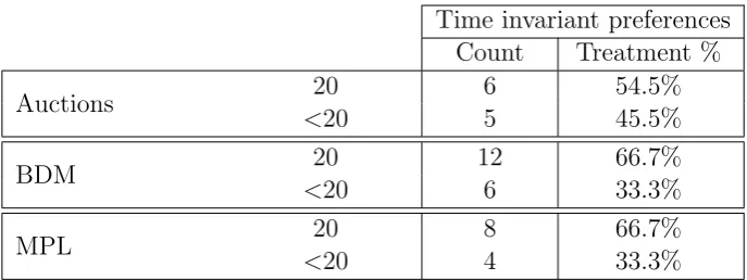
Time invariant preferences Count Treatment %

Auctions 20 6 54.5%

<20 5 45.5%

BDM _<20 12 66.7%

20 6 33.3%

MPL 20 8 66.7%

<20 4 33.3%

Table 5: Time invariant preference by treatment

subjects who exhibit non monotonic time preferences (either in “hump” or “bowl” form), which we are unable to rationalise within any of the existing models. Interestingly, this percentage is substantially larger in the MPL (23.4% of participants) elicitation method - which one might have thought of as more intuitive - than in the BDM or Auction (both 12.5%).

In addition, some agents show constant time preference profiles, i.e. they make the same declaration regardless of the time horizon. Of these, more than half (26 out of 41 subjects) always declare a value of 20, which is compatible with a unitary discount factor, and for this reason we group them together with the other ‘rational’ TIM agents. Those whose elicited values do not vary with the time horizon but are smaller than 20 are grouped together with the TIPs, as they fit the definition of weakly decreasing declared values (with a large fall for the first time horizon, which then remains constant). Their distribution by treatment is recorded in Table 5.

significant are driven by the subgroup of ‘rational’ TIMs.

For TIMs the ordering of elicited values from smaller to larger is MPL<AuctionsBDM for all time horizons when looking at median and modal values. For mean values, the order between BDM and Auctions is reversed for the shortest horizon, revealing a distribution more skewed towards the origin in the case of Auctions, which appears more dispersed. If we look at each treatment separately, it is interesting to note that the differences between the values elicited for TIP and HUBO subjects are largest with the MPL method, and smallest with the BDM, while the Auction sits somewhere in the middle, irrespective of time horizon.

We report the statistics for the non monotonic participants, too, simply for information – unsurprisingly, no clear pattern emerges there; for this reason, we omit them from the subsequent analysis.

As for the other two groups, inspection of Tables 13-15 (appendix) reveals the follow-ing:

• Auction-BDM comparison: for TIM agents, the two distributions differ in location (significant at 10% for four months), variance (significant at 1% and 5%, respectively for one and two month horizons, and at 10% for four month horizon), and distri-bution (Auctions stochastically dominate BDM at 10% significance for the longest time horizon) while no statistical significance at the conventional level is detected for TIP subjects (see summary in Table 7);

• BDM-MPL: the two distribution differ in variance for TIM subjects but not for the TIPs; differences in location and other general differences that we saw for aggregate data appear to obtain as the combination of disaggregated differences that emerge within each of the two subpopulations for different time horizons (see summary in Table 8)

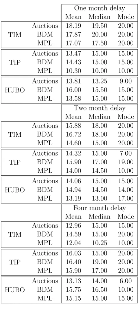
One month delay Mean Median Mode

TIM

Auctions 18.19 19.50 20.00 BDM 17.87 20.00 20.00 MPL 17.07 17.50 20.00

TIP

Auctions 13.47 15.00 15.00 BDM 14.43 15.00 15.00 MPL 10.30 10.00 10.00

HUBO

Auctions 13.81 13.25 9.00 BDM 16.00 15.50 15.00 MPL 13.58 15.00 15.00

Two month delay Mean Median Mode

TIM

Auctions 15.88 18.00 20.00 BDM 16.72 18.00 20.00 MPL 14.60 15.00 20.00

TIP

Auctions 14.32 15.00 7.00 BDM 15.90 17.00 19.00 MPL 14.00 14.50 10.00

HUBO

Auctions 14.06 15.00 15.00 BDM 14.94 14.50 14.00 MPL 13.19 13.00 17.00

Four month delay Mean Median Mode

TIM

Auctions 12.96 15.00 15.00 BDM 14.59 15.00 20.00 MPL 12.04 10.25 10.00

TIP

Auctions 16.03 15.00 20.00 BDM 16.40 19.00 20.00 MPL 15.90 17.00 20.00

HUBO

Auctions 13.13 14.00 6.00 BDM 15.75 16.50 10.00 MPL 15.15 15.00 15.00

Auctions vs. BDM

TIMs TIPs

location One month o o

Two Months o o

Four Months * o

variance One month *** o

Two Months ** o

Four Months o o

general One month o o

(one sided) Two Months o o Four Months *(Auctions-MPL) o

Legend (significance value) ***: 1%, **: 5%, *: 10%,

o: statistics p-value is greater than 10%

Table 7: Summary of differences between distributions of elicited values

Summing up, then, it appears that subjects whose money discount rates have a more standard behaviour, in that they fall as the time horizon increases, are more sensitive to the framing of the elicitation method that subject with less standard time preference profiles. This is all the more puzzling if we consider that TIMs also seem to be more ’on the ball’ than TIPs when it comes to awareness of the interest rates corresponding to their declaration, as we explain in the next section.

Auctions vs MPL

TIMs TIPs

location One month * **

Two Months * o

Four Months o o

variance One month *** o

Two Months o o

Four Months * o

general One month **(MPL-Auctions) **(MPL-Auctions) (one sided) Two Months *(MPL-Auctions) o

Four Months o o

Legend (significance value) ***: 1%, **: 5%, *: 10%,

o: statistics p-value is greater than 10%

BDM vs MPL

TIMs TIPs

location One month o ***

Two Months ** **

Four Months ** o

variance One month ** o

Two Months *** o

Four Months ** o

general One month o ***(MPL-BDM) (one sided) Two Months *(MPL-BDM) o

Four Months **(MPL-BDM) o

Legend (significance value) ***: 1%, **: 5%, *: 10%,

o: statistics p-value is greater than 10%

Table 8: Summary of differences between distributions of elicited values

4.3

Errors

As anticipated, after eliciting the money discount rates, in the last phase of the experiment we verified (in an incentive compatible way) how aware subjects were of the interest rates implied by their choices. In a nutshell, we find that TIMs make errors which are in absolute value closer to zero than TIPs, and that the latter tend to overestimate the rates corresponding to their choices (i.e. they are biased in one direction). Interestingly, the elicitation method seems to have no effect on mistakes. Let us consider these points in more detail.

We begin by showing the frequency of mistakes by time horizon, reported in Table 10 What is immediately evident is that many more TIMs than TIPs guess their implied rates correctly (for responding TIMs guesses within 10% are roughly 28%, 21% and 13% for one, two and four month horizons, while for TIPs we have 13%, 8% and 15%, re-spectively), though for TIMs mistakes increase with the time horizon. For both TIMs and TIPs most of the correct guesses are within 5% of the true implied rates, and non respondents are roughly 17% for both groups.

Profile of time preferences

Hump-Bowl Time Is Money Time Is Pleasure

One month Don’t know 6 20 8

Error >10% 22 69 34 5%<Error10 % 0 1 1

Error 5% 1 26 4

Two months Don’t know 8 20 9

Error >10% 21 76 35 5%<Error10 % 0 2 1

Error 5% 0 18 2

Four months Don’t know 7 19 7 Error >10% 22 84 34 5%<Error10 % 0 1 1

Error 5% 0 12 5

Table 10: Frequency of mistakes by time horizon

the choice), differences between TIM and TIP subjects are always statistically significant, although while for short time horizons TIPs make larger mistakes, it is TIMs who make larger mistakes for the four month horizon. However there may be a confounding effect: by definition, TIMs are those subjects for whom declared values decrease with time horizon, whereas the opposite is true for TIPs. So if errors grow with the distance from the undiscounted sum, one would find spurious differences due to the size of the errors, not to other specific cognitive biases.

To address this point we look at the whole series of differences/correct answers, without distinguishing by time horizon. Indeed in this case we find significant differences, as follows (where of course we are excluding subjects who did not provide an answer for the rates):

1. A Fisher exact test18

shows association between type of agent (TIMs vs TIPs) and ‘propensity’ to make mistakes;

2. When looking at signed differences between actual and declared rates, this difference is significant at 10% with WMW19

and at 1% for KS (which does not assume that

18

The two sided p-value for a Fisher test of the independence of the errors (within or without 10% of true value) in the two populations of TIMs and TIPs (Table 11) has a two sided exact p-value of 0.0238. The one sided exact p-value testing independence against the alternative that the proportion of correct guesses is larger for TIMs than for TIPs is 0.0127.

19

the distributions are the same), and shows that the distribution for TIPs first order stochastically dominates20

the one for TIMs: that is, TIPs tend tooverestimate the rates (the formula for the errors is “true rate – declared rate”);

3. When looking at absolute differences, both WMW21

and KS22

show a significant difference between the two populations of agents; now it is the TIMs who first order stochastically dominate the TIPs, i.e. TIMs make errors which are closer to zero than TIPs.

Below we look at these three last points more in detail. First of all, consider the distri-bution of guesses within 10% of the correct from Table 11.

TIMs TIPs Total More than 10% error 229 103 332 away from correct rate (79.24%) (88.03%)

Within 10% 60 14 74

of correct rate (20.76%) (11.97%)

Total 289 117 406

Table 11: Frequency of mistakes by preference profiles regardless of time horizon

This table shows that there are almost twice as many rational subjects who get within 10% of the correct guess (in proportion) as compared to TIPs. These differences are statistically significant: the one sided Fisher’s exact test rejects the null hypothesis of equality of success rates against the alternative that the success rate is higher in the TIM population as compared to the TIPs. If we then look at the differences and absolute differences between correct and guessed rates, we find that TIPs tend to overestimate the rates as compared to rational subjects, and also to make larger mistakes (see Figures 6a and 6b).

20

The Kolmogorov Smirnov test comparing the differences between actual and declared rates in the two populations of TIMs and TIPs rejects the null against the one sided alternative that errors by TIPS first order stochastically dominate errors by TIMs has an exact p-value of 0.006.

21

The Wilcoxon-Mann-Withney rejects the null that the two distributions come from the same

popula-tion against the one sided alternative that errors are inabsolute value larger for TIPs at 10% confidence

level (exact p-value 0.0006).

22

(a) Signed rate estimation error (b) Absolute rate estimation errors

Figure 6: Distributions of the rate estimation error

pothesis of equal distribution in favour of the alternative hypothesis that the distribution of errors for TIPs first order stochastically dominates the one for TIMs: that is, TIP sub-jects’ errors are more concentrated on larger negative values than those of TIM subjects, indicating that TIPs tend to overestimate the effective rates. If we then turn to consider the absolute size of the mistakes to abstract from over or under estimation of the errors, a KS test rejects the null hypothesis of equality in favour of an alternative where now it is the distribution of errors for TIMs that first order stochastically dominates the one for TIPs: that is, TIMs tend to make smaller errors, regardless of sign, as compared to TIPs.

Finally, observe how these differences change across treatments:

Auctions BDM MPL Time is Money outside 10% 69 (71.9%) 79 (84.1%) 81 (81.8%)

within 10% 27 (28.1%) 15 (15.9%) 18 (18.2%) Time is Pleasure outside 10% 27 (70.1%) 40 (95.3%) 36 (93.3%)

within 10% 11 (29.9%) 2 (4.7%) 1 (2.7%)

Table 12: Subjects and errors by treatment

Auctions is particularly interesting, as these were the closest methods in terms of visual layout.

5

Concluding remarks

The general conclusion we draw from the experimental results is that in ‘competitive’ situations (either against Nature, as in the BDM mechanism, or against other human players, as in an auction), subjects behave differently than when compiling a table, al-though decision-theoretically all situations are equivalent.23

This is worrisome for the external validity of standard elicitation methods, since competitive situations are at least as common in real life as non competitive ones.

Drilling into our results further, we have categorised subjects into three main groups based on the time monotonicity of the elicited values, and found that the proportion of subjects displaying non-standard choice behaviour is non-negligible. Interestingly, the differences across treatments appear to be driven by the choices of the ‘TIM’ subjects, i.e. those who, in accordance to the standard time preference framework, are prepared to pay more to speed-up receipt of a prize the longer the delay. Why could this be? Our experiment is exploratory in nature, and was not designed to test specific explanations for the (unanticipated) observed results. However, we note that they are compatible with the assumption that decision makers not relying on heuristics are more easily influenced by a change in the framing of the problem. As explained at length in the paper, the three elicitation methods have been constructed to make them equivalent and to provide the same incentives both on and off the optimal behaviour, so that any differences in observed behaviour can only be down to the payoff irrelevant presentation of the questions. It is conceivable that a decision maker relying on heuristics will be less prone to being influenced by the frame. Compatible with this line of reasoning is the fact that ‘TIP’ subjects (i.e. those who appear to like delays) do make larger errors in assessing their choices ex post: whether or not wrong-guessing the rate of return implied by each choice is down to imperfect recall, lack of attention or low computational abilities (or to something else), a decision maker relying on simple heuristics may be less likely to base his choices on rate of returns.

Perhaps contrary to expectations, subjects are more impatient in non-competitive situations (see table 6), regardless of time preference profile. However, these results can

23

also be couched in the context of differences between choice and matching tasks. As discussed in the introduction, such differences have been uncovered in various domains:24

possible explanations go from emotional distress25

to the fact that, when attributes of the objects being evaluated are clearly recognizable, choice tasks attribute more weight to the more important attributes that do matching task (prominence effect).26

Note, though, that these are all within-subject designs, i.e. the same subject is confronted with both choice and matching tasks. Once the connection between the two is made less clear, the choice-matching discrepancy should disappear, as shown in e.g. Fischer et al [12]. Thus with a between-subject design like the one we have employed, one should expect to observe no significant differences across elicitation method (provided, of course, that the subject in each treatment have been drawn from the same subject pool). Moreover, our finding is in the context of incentive compatible, real reward choices, not hypothetical ones. Yet we do find these differences, which leaves wide open the question of why they occur.27

Since the estimation of discount factors depends on the reliability of the time preference elicitation method, we hope that our contribution will open up further lines of research in the investigation of the relative merits of elicitation techniques other than the (so far most widely used) multiple price list format.

References

[1] Mazar, Nina, Botond K¨oszegi and Dan Ariely (2014) “True Context-Dependent Pref-erences? The causes of Market-Dependent Valuations”, Journal of Behavioral

Deci-sion Making, 27 (3): 200–208. 23

[2] Anand, P., P. Pattanaik and C. Puppe, eds., (2009)Handbook of Rational and Social

Choice, Oxford University Press, Oxford.

[3] Andersen, S., G. W. Harrison, M. I. Lau and E. E. Rutstr¨om (2006) “Elicitation using multiple price list formats”, Experimental Economics, 9: 383-405. 14

24

See e.g. the seminal paper by Tversky, Sattath and Slovic [40].

25

See Luce, Payne and Bettman [24].

26

See e.g. Fischer et al. [12].

27

[4] Andersen, S., G. W. Harrison, M. I. Lau and E. E. Rutstr¨om (2008) “Eliciting Risk and Time preferences”, Econometrica, 76 (3): 583-618.

[5] Becker, G. M., M. H. DeGroot, and J. Marschak (1964) “Measuring utility by a single-response sequential method”,Behavioral Science, 9: 226-232 1

[6] Benhabib, J., A. Bisin and A. Schotter (2010) “Present-bias, quasi-hyperbolic dis-counting, and fixed costs”, Games and Economic Behavior, 69 (2): 205-223. 3, 8 [7] Braga, Jacinto and C. Starmer (2005) “Preference anomalies, preference elicitation

and the dicovered preference hypothesis”, Environmental and Resource Economics, 32: 55-89. 27

[8] Casari, Marco and Davide Dragone (2011) “On negative time preferences”,

Eco-nomics Letters, 111(1): 37-39. 10

[9] Coller and M. Williams (1999) “Eliciting Individual Discount Rates”, Experimental

Economics, 2: 107-127. 8

[10] Cubitt, R. and D. Read (2007) “Can Intertemporal Choice Experiments Elicit Time Preferences for Consumption”,Experimental Economics, 10(4): 369-389. 2

[11] Thomas Dohmen, Thomas, Armin Falk, David Huffman and Uwe Sunde (2012) “In-terpreting Time Horizon Effects in Inter-Temporal Choice,” IZA Discussion Papers 6385, Institute for the Study of Labor (IZA). 1, 12

[12] Fischer, G. W., Z. Carmon, D. Dan Ariely and G. Zauberman (1999) “Goal-based Construction of Preferences: Task Goals and the Prominence Effect”, Management

Science, 45(8): 1057-1075. 5, 26

[13] Frederick, S., G. Loewenstein and T. O’Donoghue (2002) “Time discounting and time preferences: a critical review”, Journal of Economic Literature, vol. 40: 351-401. 1 [14] Halevy, Yoram (2014) “Time Consistency: Stationarity and time Invariance”, mimeo,

University of British Columbia 2

[16] Harrison, G. (1992) “Theory and Misbehavior of First Price Auctions: Reply”,

Amer-ican Economic Review, 82: 1426-1443. 1, 2

[17] Harrison, G., M. Lau and M. Williams (2002) “Estimating Individual Discount Rates in Denmark: A Field Experiment.” American Economic Review 92: pp. 1606-1617. 2

[18] Harrison, G., M. Lau and E. Rutstr¨om (2004) “Experimental Methods and Elicitation of Values”, Experimental Economics, 7(2): 123-140. 1

[19] Horowitz, J. K. (1991) “Discounting money payoffs: an experimental analysis”, in S. Kaish and B. Gilad (Eds.),Handbook of Behavioral Economics (vol 2B, pp. 309-324), Greenwich, CT, JAI Press. 4

[20] Kirby, K. N. (1997) “Bidding on the future: Evidence against normative discounting of delayed rewards”, Journal of Experimental Psychology: General, 126: 54-70. 4 [21] Kirby, K. N. and N. Marakovich (1995) “Modeling Myopic Decisions: Evidence for

Hyperbolic Delay-Discounting within Subjects and Amounts”, Organizational

Be-havior and Human Decision Processes, 64: 22-30. 4

[22] Lee, K. and M. C. Ashton (2008) “The HEXACO Personality Factors in the Indige-nous Personality Lexicons of English and 11 Other Languages”, Journal of

Person-ality, 76: 1001-1054. D

[23] Lichtenstein, S., and P. Slovic (1971) “Reversals of preferences between bids and choices in gambling decisions”, Journal of Experimental Psychology, 89: 46–55. 7 [24] Luce, M. F., J. W. Payne and J. R. Bettman (1991) “Emotional Trade-Off Difficulty

and Choice”, Journal of Marketing Research, 36: 143-159. 25

[25] Manzini, P. (2001), “Time preferences: do they matter in bargaining?”, Working Paper n. 445, Department of Economics, Queen Mary, University of London. 3

[26] Manzini, P. and M. Mariotti (2006) “Two-stage boundedly rational choice procedures: Theory and experimental evidence”, QM Working Paper n.561/200.

[28] Manzini, P., M. Mariotti and L. Mittone (2010) “Choosing monetary sequences: theory and experimental evidence”, Theory and Decision, 65 (3): 327-354.

[29] Noor, Jawwad (2011) “Hyperbolic Discounting and the Standard Model: eliciting discount functions”, Journal of Economic Theory, 144 (5): 2077-2083. 2

[30] Noussair, C., S. Robin and B. Ruffieux (2004) “Revealing consumers’ willingness-to-pay: A comparison of the BDM mechanism and the Vickrey auction”, Journal of

Economic Psychology, 25: 725-741. 6, 9

[31] Filiz-Ozbay, Emel, Jonathan Guryan, Kyle Hyndman, Melissa Kearney, Erkut Ozbay, 2013, “Do Lottery Payments induce savings behavior? Evidence from the Lab”, mimeo, Univeristy of Maryland 2

[32] Plott, C. R. (1996) “Rational individual behavior in markets and social choice pro-cesses: the discovered preference hypothesis”, in K. Arrow, E. Colombatto, M. Perle-man ad C. Schmidt (Eds.)Rational Foundations of Economic Behavior (pp. 225-250), MacMillan, London. 27

[33] Plott, C. R., and K. Zeiler (2005) “The Willingness to Pay–Willingness to Accept Gap, the ‘Endowment Effect’, Subject Misconceptions, and Experimental Procedures for Eliciting Valuations”, American Economic Review, 95: 530-545. 15

[34] Plott, C. R., and K. Zeiler (2005), appendix to “The Willingness to Pay–Willingness to Accept Gap, the ‘Endowment Effect’, Subject Misconceptions, and Experi-mental Procedures for Eliciting Valuations”, available online at http://www.e-aer.org/data/june05 app plott.pdf 15

[35] Read, D., M. Airoldi and G. Loewe (2005) “Intertemporal tradeoffs priced in interest rates and amounts: A study of method variance” LSEOR working paper.

[36] Read, D. and R. Roelofsma (2003) “Subadditive versus hyperbolic discounting: A comparison of choice and matching ”,Organizational Behavior and Human Decision

Processes, 91: 140-153. 1

[37] Rutstr¨om, E. (1998) “Home-grown values and incentive compatible auction design”,

[38] Shogren, Jason F., Sungwon Cho, Cannon Koo, John List, Changwon Park, Pablo Polo and Robert Wilhelmi (2001) “Auction mechanisms and the measurement of WTP and WTA”, Resource and Energy Economics, 23 (2): 97-109. 6

[39] Tokarchuk, O. (2007) “The effect of representation mode on elicited individual dis-count rates”, DISA Working paper n. 121, University of Trento 8

Appendices

A

Instructions

The translation of the original instructions (in Italian) follows below (we omit the compre-hension test for space reasons - it showed three screens, one for each time horizon, as filled by an hypothetical participants. On each screen two simple questions asked about what payment would the hypothetical participant received if drawn or not drawn. Screenshots are availablehere.

A.1

Sheet 1 (common to all treatments)

This experiment studies choice over time. Please read carefully the instructions that follow while an assistant also reads them aloud. You will be given a fixed participation fee at the end of the experiment. Moreover you may be able to receive an additional sum on top of the participation fee. This additional amount will depend on your choices and on a random draw. More precisely, you will have one chance in two to be drawn to receive the additional payment.

At the end of the experiment we will ask you to complete a questionnaire. The information collected will be used solely for research purposes. The information collected will be kept completely anonymously.

Click ‘NEXT’ to continue.

A.2

Sheet 2

A.2.1 - MPL

TAKING PART IN THE EXPERIMENT

Option A instead is different on all rows, and varies between a minimum of e_{0.50 and a}

maximum of e_{20. Careful! You must make a choice in each row. To do so you will have}

to use the cursor in the middle of the screen: you can scroll it using the mouse to select the option that you prefer in each row. You will see three tables in total, differing from one another only for the delay with which thee_{20 of option B are payable.}

Three random draws will take place at the end of the experiment. The first will draw one of the three screens, the second will draw one of the forty rows from that screen, and the third will draw the participants which will receive the additional payment, corresponding to the choice made in the row drawn. This means that if you are drawn to receive a payment, the amount of money you will receive will be that corresponding to the option (A or B) that you chose in the row drawn. This means that each choice you will make in each of the three tables may be rewarded.

Click ‘NEXT’ to continue

A.2.2 Auctions

TAKING PART IN THE EXPERIMENT

By participating in this experiment you have one chance in two of being drawn to receive e_{20, which will be payable with a delay of some weeks. However you will have}

the opportunity to anticipate receipt to tomorrow. In this case you will have to give up part of the total amount. Very shortly you will see a screen where you will be able to take part in an auction to anticipate the payment to tomorrow. As the other participants, you will have to declare the minimum amount you are prepared to receive in place of the full e_{20 to receive your payment tomorrow, entering a value between} e_{0.50 and} e_{20 in} e_{0.50 steps. The participant declaring the lowest value will acquire the right to receive}

the payment earlier. If two or more participants have inserted the same minimum value, all of these participants will acquire the right to receive the payment earlier.

How much is the early payment?

If you are drawn for payment:

1) if your declared value is the smallest, you will be entitled to receive tomorrow an amount of money equal to the lowest of all the other declarations excluding yours. Thus in case of a draw with one or more participants, such lowest value will be the same as the one you declared.

2) if your declared value is not the smallest, you will be entitled to the full e_{20 but}

with delay.

John who declares e_{y, and suppose that they are both drawn to receive payment. If} e_x

is smaller than e_{y, Jane gets the right to early payment, and will receive} e_{y tomorrow,}

while John will receivee_{20 with delay; if}e_{x is larger than}e_{y, Jane will receive} e_{20 with}

delay while John gets the right to early payment, and will receive e_{x tomorrow; if} e_x

and e_{y are the same, then both Jane and John will receive} e_x=e_{y tomorrow.}

How much to declare?

If you think about it, you will see that the best option for you is to declare the amount that makes you indifferent between receiving such amount tomorrow or the whole e₂₀

with delay. Consider for instance the two extreme values, namely e_{0.50 and} e_{20. If}

you declare e_{0.50, you will be sure that, if drawn for payment, you will receive your}

payment tomorrow, but you could earn as little ase_{0.50 in case another participant has}

also declared e_{0.50. If you declare} e_{20 you will be sure that, if drawn, you will receive}

the whole e_{20 albeit with delay: the exception is if everybody else has also declared}e_20,

in which case everybody will have the right to early payment. Yet even in this case if the declaration which makes you indifferent is less than e_{20, by declaring such value you}

would be the only participant to get the right for early payment, and would receive e₂₀

tomorrow anyway.

You will be shown three screens in total, which differ only for the delay with which the full e_{20 are payable.}

Two random draws will take place at the end of the experiment. The first will draw one of the three screens, the second will draw the participants who will receive a payment corresponding to the choices made. This means that if you are drawn to receive a payment, the amount of money you will receive will be based on the choice you made in the screen drawn. This means that each choice you will make in each of the three screens may be rewarded.

Click ‘NEXT’ to continue

A.2.3 BDM

TAKING PART IN THE EXPERIMENT

By participating in this experiment you have one chance in two of being drawn to receivee_{20, which will be payable with a delay of some weeks. However you will have the}

opportunity to anticipate receipt to tomorrow. In this case you will have to give up part of the total amount. Very shortly you will see a screen where you will be able to declare the minimum amount you are prepared to receive in place of the fulle_{20 to receive your}

choice a number between e_{0.50 and} e_{20 in} e_{0.50 increments will be drawn at random.}

Every value betweene_{0.50 and}e_{20 in}e_{0.50 increments has the same probability of being}

drawn

How much is the early payment?

If you are drawn for payment:

1) if your declared value smaller or equal to the one drawn, you will be entitled to receive tomorrow an amount of money equal to the number drawn.

2) if your declared value is larger than the one drawn, you will be entitled to the full

e_{20 but with delay.}

How much to declare?

If you think about it, you will see that the best option for you is to declare the amount that makes you indifferent between receiving such amount tomorrow or the whole e₂₀

with delay. Consider for instance the two extreme values, namely e_{0.50 and} e_{20. If you}

declaree_{0.50, you will be sure that, if drawn for payment, you will receive your payment}

tomorrow, but you could earn as little as e_{0.50 in case the number drawn is} e_{0.50. If}

you declare e_{20 you will be sure that, if drawn for payment, you will receive the whole} e_{20 albeit with delay: the exception is if} e_{20 is drawn, in which you would receive} e₂₀

tomorrow. Yet even in this case if the declaration which makes you indifferent is less than

e_{20, by declaring such value you would receive} e_{20 tomorrow anyway.}

You will be shown three screens in total, which differ only for the delay with which the full e_{20 are payable.}

Three random draws will take place at the end of the experiment. The first will draw one of the three screens, the second will draw a number between e_{0.50 and} e_{20 in} e_{0.50 increments, and the third will draw the participants who will receive a payment}

corresponding to the choices made. This means that if you are drawn to receive a payment, the amount of money you will receive will be based on the choice you made in the screen drawn. This means that each choice you will make in each of the three screens may be rewarded.

Click ‘NEXT’ to continue

A.3

Sheet 3

A.3.1 MPL

INTEREST RATE PHASE

In each of the previous screens your choices have determined the last line (counting from the top) in which you have chosen option A over option B. On that row of course the value of option A would have been between e_{20 (if you chose option A only on the}

first line, the one at the top) and e_{0.50 (if you chose option A always, down to the}

bottom line). In the next screen we will ask you to enter the simple annual interest rate corresponding to the choice you made in the last line where you chose option A, in each of the three tables.

If drawn, your earnings will be determined as follows:

1. if the simple annual interest rate you entered for the table drawn is within ±5% of the simple annual interest rate corresponding to your choice, you will earn e_2;

2. if the simple annual interest rate you entered for the table drawn differs more than

±5% but not more than ±10% from the simple annual interest rate corresponding to your choice, you will earn e_1;

3. for larger differences, or if you do not enter any value, you will earn nothing.

Click on ‘NEXT’ to continue

A.4

Auctions and BDM

INTEREST RATE PHASE

In the next screen you will have the possibility, if drawn, to earn additional money. We will ask you to enter the three simple annual interest rates corresponding to the choices you made in the three preceding screens.

If drawn, your earnings will be determined as follows:

1. if the simple annual interest rate you entered for the version drawn is within ±5% of the simple annual interest rate corresponding to your choice, you will earn e_2;

2. if the simple annual interest rate you entered for the version drawn differs more than

±5% but not more than ±10% from the simple annual interest rate corresponding to your choice, you will earn e_1;

3. for larger differences, or if you do not enter any value, you will earn nothing.

B

Truth-telling elicitation

B.1

MPL

Figure 7: Truthtelling payoff in the MPL method

Lets⇤ _{be the ‘true’ switching value, i.e.}

the value that makes the agent indif-ferent between receiving s⇤ _earlier

(op-tionA) and waiting for the full amount (option B). A standard rational agent would choose optionAin all those rows in which option A pays an amount s such that s > s⇤_{, and option B in all}

other rows. Number all the rows in the table progressively by the valueswhich in optionAin that particular row, iden-tifying the ‘switching row’s⇤ _{as the one}

such that the subject would chooses op-tion A in all rows with s > s⇤_{, and optionB in all other rows such that s < s}⇤_.

Figure 8: Payoffs in case of deviation from truthtelling, MPL

amount s sooner. If instead the s is less than s⇤_{, the agent will receive the option B.} At the switching row, being indifferent the decision maker could state either optionA or option B, as they are payoff equivalent. The payoff in case of truthtelling is depicted in figure 7. Based on this, it is easy to construct payoffs in case of deviations, depicted in figure 13: by deviating to a lower switching values0 _{the agent risks ending up with a lower}

payoff in case a row where values in option A falling in the interval [s0_{, s}⇤_{) is drawn; and}

similarly, deviating to a higher switching point s00 _{again the agent risks ending up with a}

(dispreferred) option B in case a row falling in the interval (s⇤_{, s}00_{] is drawn (Figure 8).}

B.2

Second price Auctions

Figure 9: Truthtelling payoff, Auctions

In a second price auction truthful rev-elation of one’s (perceived) true valua-tion is a weakly dominant strategy. A strategy for the subject consists in stat-ing an amounts.

Under truthful revelation, the sub-ject declares the amounts⇤ _{that makes}

him indifferent between receiving s⇤

sooner (denote this option by (s⇤_,0))

and the full amount L later (which we denote by (L,1)). The payoff in case of truthtelling is depicted in fig-ure 9, where on the horizontal axis we measure the minimum bid made by the competitors, and on the vertical axis the payoff accruing to the decision maker playing the auction. If prefer-ences are summarised by a utility function, the payoff derived form the two indifferent outcomes (s⇤_{,0) and (L,1) should yield the same utility, i.e. u(s}⇤_{,0) = u(L,1). In}

fig-ure 9 the light dashed grey line represents the decision maker’s utility for money under truthful revelation. Consider the case when the agent bids his true valuation s⇤_{. If the}

minimum bid is below s⇤_{, the agent is going to lose the auction, and receive the full}

and receive that second bid amount earlier, explaining the increasing portion of his utility function to the right of s⇤_{. Note that in case of a tie the second lowest bid coincides with}

s⇤_.

Figure 10: Payoffs in case of deviation from truthtelling, Auctions

on the left, the solid black locus depicts the payoff in case of overstating one’s true value, whereas the payoff when understating the true value is represented by the solid black locus on the right hand side.

B.3

BDM

For a standard agent endowed with a utility function for money, incentives are as in the auctions, as depicted in figure 11, where again the horizontal axis measures monetary amounts. Payoffs now depend not on the minimum bid, but on the number drawn. As before, utility for money is represented by the dashed light grey line, while the solid black line represents the payoff in case of truthtelling when the BDM mechanism is applied. If an individual states truthfully the amount s⇤ _{that solvesu(s}⇤_{,0) =u(L,1), then for any}

number drawn which is smaller than or equal to s⇤_{, the decision maker will receive the}

receives an amount equal to the number drawn sooner, so that his payoff now follows the dashed line.

To show that there are no incentives to deviate from truthtelling, consider the panels in figure 8, where on the left we consider deviations tos0 _{< s}⇤_{, and on the right tos}0 _{> s}⇤_.

In the left panel, while nothing changes if the number drawn, d, is smaller than s0 _{or at}

least as large ass⇤_{, ifd2[s}0_{, s}⇤_{) then the agent is going to receive that monetary amount}

immediately, yielding a lower utility than that corresponding to declaring s⇤_{. A deviation}

to a larger amount s00 _{> s}⇤ _{is also non profitable, since as before the payoff does not}

change if eitherd > s00_ords⇤_{, while if d2[s}⇤_{, s}00_{) then payment is going to be delayed,}

yielding utility u(L,1) =u(s⇤_{,0)< u(d,0).}

Figure 11: Truthtelling payoff, BDM

C

Test statistics

In this appendix we report our test statistics. All tests have been carried out with StatX-act. Unless specified, all tests are exStatX-act. The tests we consider are the following:

• Wilcoxon-Mann-Whitney tests (assumes same distribution)

• Hodges-Lehman test estimate of the WMW shift.

• Two sample Kolmogorov-Smirnov test: is a general test for the difference of two distributions, considering differences of any kind, including location and dispersion. It is not very powerful against tests which consider specific alternatives (e.g. shift in distribution), unless a one sided alternative can be specified. In the case of a one sided test, the column Fi-Fj reports the p-values corresponding to the alterna-tive hypothesis that distribution i is stochastically smaller than distribution j, or equivalently that sample i will tend to produce smaller values than sample j.

C.1

Comparing distributions of elicited values

Tables 13-15 below report p-values of the various statistics; these are highlighted in dark grey if smaller than 5%, and in light gray if between 5% and 10% .

WMWo _{Hodges-Lehman}

Auctions-BDM 95% CI All One month 0.3365 0 [-1, 0.5] Two months 0.1257 0 [-2, 0] Four months 0.05695 -1 [-3, 0] TIM One month 0.4727 0 [0, 0]

Two months 0.2454 0 [-2, 0] Four months 0.08897 -1.5 [-4, 0] TIP One month 0.3427 0 [-4.5, 2]

Two months 0.1049 -1.5 [-5, 1] Four months 0.3129 0 [-4, 1]

Legend: o _{(one sided)}

Conovero _{Two sample KS (Auctions= 1)}

|F1−F2| F1−F2 F2−F1 All One month 0.0275M _{0.8999 0.5136 0.7228}

Two months 0.0045M _{0.5492 0.2802 1}

Four months 0.147M _{0.1349 0.0675 0.9259}

TIM One month 0.001751 0.6806 0.6913 0.352 Two months 0.04082 0.5683 0.2955 0.5644 Four months 0.2391 0.1908 0.09766 0.9327 TIP One month 0.147 0.7069 0.3826 0.6393 Two months 0.2483 0.3628 0.1838 0.8372 Four months 0.4458 0.7471 0.3849 0.795

Legend: M _{exact using Montecarlo;} o _{(one sided)}

WMWo _{Hodges-Lehman}

BDM-MPL 95% CI All One month 0.004397 2 [0, 3]

Two months 0.003695 2 [0, 4] Four months 0.05738 1 [0, 3.5] TIM One month 0.1146 0 [0, 2]

Two months 0.02083 1 [0, 4] Four months 0.02973 2 [0, 5] TIP One month 0.002339 5 [2, 6.5]

Two months 0.05273 2.5 [0, 5] Four months 0.2682 0 [-1.5, 4]

Legend: o _{(one sided)}

Conovero _{Two sample KS (BDM= 1)}

|F1−F2| F1−F2 F2−F1 All One month 0.0015M _{0.03633 1 0.01817}

Two months 0.0016M _{0.05617 1 0.02808}

Four months 0.0775M _{0.4082 1 0.2054}

TIM One month 0.02597 0.4016 0.8589 0.2047 Two months 0.008945 0.1151 1.0000 0.06229 Four months 0.01334 0.05427 1.0000 0.02603 TIP One month 0.3878 0.00536 1.0000 0.00268 Two months 0.4162 0.302 0.8585 0.1513 Four months 0.433 0.5354 0.8294 0.2715

Legend: M _{exact using Montecarlo;} o _{(one sided)}