Testing and debugging functional reactive programming

2

IVAN PEREZ,

HENRIK NILSSON,

Many types of interactive applications, including video games, raise particular challenges when it comes to testing and debugging. Reasons include de-facto lack of reproducibility and difficulties of automatically generating suitable test data. This paper demonstrates that certain variants of Functional Reactive Program-ming (FRP) implemented in pure functional languages can mitigate such difficulties by offering referential transparency at the level of whole programs. This opens up for a multi-pronged approach for assisting with testing and debugging that works across platforms, including assertions based on temporal logic, recording and replaying of runs (also from deployed code), and automated random testing using QuickCheck. The approach has been validated on real, non-trivial games implemented in the FRP system Yampa through a tool providing a convenient Graphical User Interface that allows the execution of the code under scrutiny to be controlled, moving along the execution time line, and pin-pointing of violations of assertions on PCs as well as mobile platforms.

CCS Concepts: •Software and its engineering→General programming languages;Functionality; • Human-centered computing→ Graphical user interfaces;

Additional Key Words and Phrases: Functional Reactive Programming, game programming, testing, debugging, temporal logic

ACM Reference format:

Ivan Perez and Henrik Nilsson. 2017. Testing and Debugging Functional Reactive Programming.Proc. ACM Program. Lang.1, 1, Article 2 (September 2017), 27 pages.

https://doi.org/http://dx.doi.org/10.1145/3110246

1 INTRODUCTION

Testing software thoroughly is hard in general [Whittaker 2000]. Testing games raises specific additional difficulties due to their interactive and real-time aspects [Lewis et al. 2010]. For example, just specifying game input so as to ensure adequate test coverage is daunting. As a result, game developers often leave much of the testing to testers and even players. Another difficulty is the lack of reproducibility: in general, the exact same input may produce different results at different times. This is due to both deliberate random elements in many games and the effects of interacting with a constantly changing outside world at points in time that are difficult to control exactly due to real-time considerations. Consequently, the conditions that led to a bug can be hard to replicate. These challenges apply generally, regardless of what language is used to implement a game. Thus, while using a pure functional language can offer benefits at the level of unit testing thanks to referential transparency, just using a pure language offers few if any additional benefits over commonly used languages for game programming when it comes to testing a game as a whole.

Permission to make digital or hard copies of all or part of this work for personal or classroom use is granted without fee provided that copies are not made or distributed for profit or commercial advantage and that copies bear this notice and the full citation on the first page. Copyrights for components of this work owned by others than ACM must be honored. Abstracting with credit is permitted. To copy otherwise, or republish, to post on servers or to redistribute to lists, requires prior specific permission and/or a fee. Request permissions from permissions@acm.org.

© 2017 Association for Computing Machinery. 2475-1421/2017/9-ART2

Functional Reactive Programming (FRP) [Courtney et al. 2003; Elliott and Hudak 1997; Nilsson et al. 2002] helps express interactive software such as games declaratively in a way that arguably brings the benefits of pure functional programming to thesystem level. In this paper, we demonstrate thatArrowizedFRP in particular provides enough structure to address whole-program testing and debugging challenges such as those outlined above. Our work applies to FRP programs in general, but we put a particular emphasis on games, physical simulations, and related applications in this paper, as these tend to highlight the difficulties of interest here.

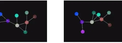
There are two sources of uncertainty in FRP programs that may affect system-level referential transparency. First, some FRP implementations use IO inside core definitions to increase versatility and performance. This makes those systems susceptible to the problems discussed earlier. Second, even if we run a simulation twice with the same initial state and user input, we may obtain different outputs if our simulations are sampled at different points in time, due to differences in system load and OS scheduling decisions outside our control, for example. This is demonstrated by the force-directed graph simulation depicted in Figure 1. This simulation does not depend on user input, yet different stable configurations are reached depending on the sampling step, due to small differences in floating point calculations.

Fig. 1. Two runs of the same graph layout algorithm in which nodes repel each other, unless directly connected, in which case they also attract. Even with identical initial conditions, two executions converge to different

stable configurations, demonstrating that pure FRPsystemsexhibit non-determinism.

Pure Arrowized FRP [Nilsson et al. 2002] completely separates all side effects and time sampling from the data processing, providing referential transparency across executions. In this variant we can truly run a program twice with the same input, poll it at the same times, and obtain the same output, enabling a form of game testing unparalleled by other languages and paradigms. Given the same architecture the results will be guaranteed by the type system and the compiler to be the same,evenacross different devices. This is a key aid for game development, especially on mobile platforms, since players often find bugs that developers cannot reproduce.

In this paper we explore how Arrowized FRP enables game testing and debugging to be ap-proached systematically in pure functional languages. The contributions of this paper are as follows: • We extend FRP constructs with a notion of temporal predicates based on Linear Temporal Logic, equipped with an evaluation function, and demonstrate how they can be used to express temporal game properties.

• We provide random input data generators, and demonstrate how they can be used effectively to test FRP games using QuickCheck.

• We present acausalsubset of Linear Temporal Logic that can be used to insert temporal assertions into FRP programs for revealing bugs during execution.

Our system works for PC, iOS and Android games implemented using the Haskell FRP framework Yampa. It is capable of recording, replaying, manipulating and visualizing execution traces from real users, as well as counter-example traces generated by QuickCheck. Our application lets us traverse an input trace and find points where assertions are violated, moving back and forth along the execution timeline and performing hot-swapping of the application to verify whether changes to the game fix existing bugs. We demonstrate the use of this setup to find bugs in real games.

2 BACKGROUND

In the interest of making this paper sufficiently self-contained, we summarize the basics of FRP and Yampa in the following. For further details, see earlier papers on FRP and Arrowized FRP (AFRP) as embodied by Yampa [Courtney et al. 2003; Elliott and Hudak 1997; Nilsson et al. 2002]. This presentation draws heavily from the summary in [Courtney et al. 2003].

2.1 Functional Reactive Programming

FRP is a programming paradigm to describe hybrid systems that operate on time-varying data. FRP is structured around the concept ofsignal, which conceptually can be seen as a function from time to values of some type:

Signalα≈Time→α

Time is (notionally) continuous, and is represented as a non-negative real number. The type parameterαspecifies the type of values carried by the signal. For example, the type of an animation would beSignal Picturefor some typePicturerepresenting static pictures. Signals can also represent input data, like the mouse position.

Additional constraints are required to make this abstraction executable. First, it is necessary to limit how much of the history of a signal can be examined, to avoid memory leaks. Second, if we are interested in running signals in real time, we require them to becausal: they cannot depend on other signals at future times. FRP implementations address these concerns by limiting the ability to sample signals at arbitrary points in time.

The space of FRP frameworks can be subdivided into two main branches, namely Classic FRP [El-liott and Hudak 1997] and Arrowized FRP [Nilsson et al. 2002]. Classic FRP programs are structured around signals or a similar notion representing internal and external time-varying data. In contrast, Arrowized FRP programs are defined using causal functions between signals, orsignal functions, connected to the outside world only at the top level.

Arrowized FRPyieldsmodular, declarative and efficient code. Pure Arrowized FRP separates IO from the FRP code itself, making the latter referentially transparentacross executions. In the following, we turn our attention to Arrowized FRP as embodied by Yampa, and later explain current limitations that our framework addresses.

2.2 Fundamental Concepts

Yampa is based on two concepts:signalsandsignal functions. A signal, as we have seen, is a function from time to values of some type, while asignal functionis a function fromSignaltoSignal:

Signalα≈Time→α

SFα β ≈Signalα→Signalβ

f

(a)arr f

g f

(b)f ≫g

f

g

(c)f &&&g

f

(d)loop f

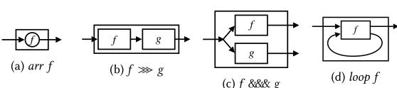
Fig. 2. Basic signal function combinators.

In order to ensure that signal functions are executable, we require them to becausal: The output of a signal function at timetis uniquely determined by the input signal on the interval [0,t].

2.3 Composing Signal Functions

Programming in Yampa consists of defining signal functions compositionally using Yampa’s library of primitive signal functions and a set of combinators. Yampa’s signal functions are an instance of the arrow framework proposed by Hughes [Hughes 2000a]. Some central arrow combinators arearr that lifts an ordinary function to a stateless signal function, composition≫, parallel composition &&&, and the fixed point combinatorloop. In Yampa, they have the following types:

arr ::(a→b)→SF a b

(≫) ::SF a b →SF b c→SF a c (&&&)::SF a b →SF a c→SF a(b,c) loop ::SF (a,c) (b,c)→SF a b

We can think of signals and signal functions using a simple flow chart analogy. Line segments (or “wires”) represent signals, with arrowheads indicating the direction of flow. Boxes represent signal functions, with one signal flowing into the box’s input port and another signal flowing out of the box’s output port. Figure 2 illustrates the aforementioned combinators using this analogy. Through the use of these and related combinators, arbitrary signal function networks can be expressed.

2.4 Time-Variant Signal Functions: Integrals and Derivatives

Signal Functions must remain causal and leak-free, and so Yampa introduces limited ways of depending on past values of other signals. Integrals and derivatives are important for application domains like games, multimedia and physical simulations, and they have well-defined continuous-time semantics. Their types in Yampa are as follows (vrepresents the type of vectors, andsthe type of scalars):

integral ::VectorSpace v s⇒SF v v derivative::VectorSpace v s⇒SF v v

Time-aware primitives like the above make Yampa specifications highly declarative. For example, the position of a falling mass starting from a positionp0 with initial velocityv0 is calculated as:

fallingMass::Double→Double→SF()Double fallingMass p0 v0=arr (const(−9.8))

≫integral≫arr(+v0)

≫integral≫arr(+p0)

This resembles well-known physics equations (i.e. “the position is the integral of the velocity with respect to time”) even more when expressed using Paterson’s Arrow notation [Paterson 2001]:

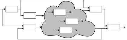
Fig. 3. System of interconnected signal functions with varying structure

v←arr(+v0)≪integral−≺(−9.8) p←arr(+p0)≪integral−≺v returnA−≺p

2.5 Events and Event Sources

To model occurrences at discrete points in time, Yampa introduces theEventtype:

dataEvent a=NoEvent|Event a

A signal function whose output signal is of typeEvent T for some typeTis called anevent source. The value carried by an event occurrence may be used to convey information about the occurrence. The operatortagis often used to associate such a value with an occurrence:

tag::Event a→b→Event b

2.6 Switching

The structure of a Yampa system may evolve over time. These structural changes are known as mode switches. This is accomplished through a family ofswitchingprimitives that use events to trigger changes in the connectivity of a system. The simplest such primitive isswitch:

switch::SF a(b,Event c)→(c→SF a b)→SF a b

Theswitchcombinator switches from one subordinate signal function into another when a switching event occurs. Its first argument is the signal function that is active initially. It outputs a pair of signals. The first defines the overall output while the initial signal function is active. The second signal carries the event that will cause the switch to take place. Once the switching event occurs, switchapplies its second argument to the value tagged to the event and switches into the resulting signal function.

Yampa also includesparallelswitching constructs that maintaindynamic collectionsof signal functions connected in parallel [Nilsson et al. 2002]. Signal functions can be added to or removed from such a collection at runtime in response to events, whilepreservingany internal state of all other signal functions in the collection (see Fig. 3). The first class status of signal functions in combination with switching over dynamic collections of signal functions makes Yampa an unusually flexible language for describing hybrid systems.

2.7 Animating Signal Functions

reactimate::IO(DTime,a)→(b→IO())→SF a b→IO()

The functionreactimateapproximates the continuous-time model presented here by performing discrete sampling of the signal function, feeding input to and processing output from the signal function at each time step. The first argument toreactimateis an IO action that will obtain the next input value along with the amount of time elapsed (or “delta” time,DTime) since the previous sample. For example, in a setting of music with CD audio quality, the delta time would be set to correspond to a system sampling frequency of 44.1 kHz, i.e. 1/44100 s, and the input could be note-on and note-off messages from a connected synthesizer keyboard. The second argument is a function that, given an output value, produces an IO action that will process the output in some way. For example, it could send sound samples to the audio subsystem for immediate playback. The third argument is the signal function to be animated.

2.8 Limitations of Current FRP Systems

FRP programs use IO to gather input data and render their output. Unlike in pure Arrowized FRP, some FRP implementations hide IO behind the scenes, and reading a signal may result in IO actions being executed [Patai 2009]. While they use low-level adjustments to guarantee that polling a signal at the same conceptual time delivers temporally consistent results across the whole program, without additional adjustments these implementations lack referential transparency across executions.

Even in IO-free forms of FRP, simply sampling a simulation at different points in time can render different results. The non-determinism introduced by the sampling policy is demonstrated by the force-directed graph simulation in pure FRP depicted in the introduction, in Figure 1. Implemented in Pure Arrowized FRP, this simulation is not interactive, but the numerical methods used to calculate forces, velocities and positions depend on the sampling time, and are highly affected by small variations. As a result, the layouts obtained when the simulation stabilizes are very dependent on the sampling step.

Because pure Arrowized FRP does separate the data processing from all side effects, including the time sampling policy, we could truly run the program twice with the exact same input and sample at the same times, obtaining the same results. This constitutes a form of referential transparency across executions suitable for complex interactive applications, especially games.

In the following we take advantage of this feature of Arrowized FRP to test and debug FRP games. We present an extension to Arrowized FRP with Temporal Propositions, and introduce two ways of using temporal properties: in a black-box manner, to test the behaviour of an FRP construct for some input data, and inside FRP programs as assertions, to monitor and debug FRP systems from the inside. We provide APIs to test these programs in a referentially transparent way, using tools like QuickCheck. We also present a debugger for Yampa games, together with an advanced GUI for live debugging that connects to running games on PC, iOS and Android devices via the network and allows controlling them, recording, replaying and manipulating input traces.

3 TEMPORAL LOGIC

Temporal Logic is a branch of Modal Logic in which propositions are quantified over time [Emerson 1990; Pnueli 1977]. Just like the value of a signal in FRP varies over time, so does the truth value of a proposition in Temporal Logic.

oftime-varying values, orfunctions of time. This will help us understand which Temporal Logic constructs can be defined in terms of FRP constructs.

3.1 Semantic Domain

In the following we will consider time abstract and assume only that it is linear (that is, that there is a total order and progresses towards the future) with a starting point denoted 0. In Temporal Logic the nature of time (bounded vs unbounded, discrete vs continuous, etc.) plays a central role, determining both which modalities can be defined and which propositions hold. In FRP, time is conceptually continuous, but always discrete during execution. We consider a temporal proposition to be a time-dependent function, that is, a boolean whose value changes over time:

TProp≡Time→Bool

3.2 Point-wise Operators

Defining the standard logical operators, likeandandnot, is straightforward:

neg:TProp→TProp negϕt = ¬¬¬ (ϕt)

and:TProp→TProp→TProp andϕ ψt=ϕt∧∧∧ψ t or:TProp→TProp→TProp orϕ ψt =ϕt∨∨∨ψ t

impl:TProp→TProp→TProp implϕ ψt=negϕt∨∨∨ψt

The previous logical operators act point-wise (or time-wise), and their meaning should be obvious. For instance,negϕis true at a timetifϕis not true at that time.

3.3 Temporal Modalities

In temporal logic we also want to define propositions that refer to other points in time, for which we define four temporal operators:always(at every point in the future),eventually(at some point in the future),history (at every point in the past), andever (at some point in the past). These correspond to the well-known Priorean operators Global, Future, History and Past [Prior 1967].

always:TProp→TProp

alwaysϕt=∀t′∈∈∈ Time((t′>t)→→→ϕt′) eventually:TProp→TProp

eventuallyϕt=∃t′∈∈∈ Time((t′>t)∧∧∧ϕt′) ever:TProp→TProp

everϕt=∃t′∈∈∈ Time((t′<t)∧∧∧ϕt′) history:TProp→TProp

historyϕt=∀t′∈∈∈ Time((t′<t)→→→ϕt′)

The above temporal operators are sometimes defined in terms of more fundamental operators, namelyUntilandNext. Until is defined as:

until:TProp→TProp→TProp

untilϕ ψt=∃t′∈∈∈ Time(t′⩾t→→→(ψt′∧∧∧ ∀t′′∈∈∈ Time(t′′<t′→→→ϕt′′)))

That is,ϕholds at every point untilψdoes.

Next expresses a temporal property that holds at the next time sample. This requires that time be discrete, which is true in our implementations, although time in FRP can be conceptually continuous. We use the functionN to refer to the successor or next time.

next:TProp→TProp nextϕt=ϕ (N (t))

The semantic domain of temporal logic, as given above, is bigger than that of FRP. While FRP Signal Functions must becausal, functions over Temporal Propositions may not be so. Modalities likealways, for example, make the present depend on the future, and thus cannot be implemented easily and efficiently in Arrowized FRP as Boolean-carrying signals. Even if we limit our attention to modalities that look only to the present or the past,history, for example, depends onall the past, which could lead to memory leaks depending on how it is implemented or evaluated.

In section 4 we present an encoding of Linear Temporal Logic withalways,eventuallyandnext modalities, which we use to test temporal predicates for a given input signal and time domain. In section 6 we introduce a causal subset of the LTL presented before that can be implemented efficiently in FRP in the form of Boolean-carrying Signals, letting us define temporal assertions checked as games run live.

4 TEMPORAL LOGIC APPLIED TO FRP

In this section we present an encoding of Linear Temporal Logic operating on Signal Function Temporal Propositions. This allows us to test temporal properties of SFs, considered as black boxes. In section 5 we use this encoding to demonstrate how to test temporal predicates using existing tools like QuickCheck. Section 6 explores the inverse question, that is, which Temporal operators can be implemented as causal FRP constructs and used to include assertions in FRP programs checked during execution.

4.1 Temporal Predicates

The following of Linear Temporal Logic allows us to look into the present and the future. We introduce a basic value constructor to make Signal Functions unapplied temporal propositions. We also provide the two fundamental temporal operatorsNextandUntil, and the two non-fundamental EventuallyandAlways, which correspond to the non-strict counterparts of the temporal modalities with the same names described in the previous section.

dataTPred awhere

Prop ::SF a Bool→TPred a

And ::TPred a→TPred a→TPred a Or ::TPred a→TPred a→TPred a Not ::TPred a→TPred a

Implies ::TPred a→TPred a→TPred a Always ::TPred a→TPred a

Until ::TPred a→TPred a→TPred a

4.2 Evaluation

To evaluate aTPredwe need to provide an input signal. Conceptually, we can think of aTPred a for some typeaas a possibly-non-causal function that takes a Signal of typeadefined on a time domain and returns a Temporal Proposition (a Signal of typeBool) on the same time domain.

In our implementation we provide both the signal and the time domain in the form of a finite inputstreamor samplestream:

typeSignalSampleStream a=(a,FutureSampleStream a)

typeFutureSampleStream a=[(DTime,a)]

SignalSampleStreamrepresents the signal starting from the first sample, always at time 0, and FutureSampleStreamrepresents streams in which the samples are spaced by strictly positive delays. We can now give an evaluation function that takes a Temporal Predicate and a sample stream and evaluates the temporal predicate at the initial time:

evalT::TPred a→SignalSampleStream a→Bool

When we evaluate aTPredby providing a stream of input samples, we are effectively restricting the time domain to a subset defined implicitly by the times of the samples in the input stream. Note that the functionevalT only lets us query the value of aTPredat the initial time, but we can always refer to specific future times usingNext.

4.3 Examples

Let us now introduce an example of an FRP program, define temporal assertions and verify them. We start with a simple animation of a falling ball, considering only the vertical axis:

fallingBall::Double→SF ()Double fallingBall p0=proc()→do

v←integral0−≺ −9.8 p←integral0−≺v returnA−≺(p0+p)

whereintegral0is an implementation of Euler integration using the rectangle rule.

To check, for example, that the position of the falling ball at any time is lower than the initial position, one can define the following property:

ballFellLower::Double→TPred()

ballFellLower p0=Prop(fallingBall p0≫arr(λp1→p1⩽p0))

We now test this property in a session, using an input streamstream01 of 42 samples spaced by 0.1 seconds, carrying no data (that is, a stream((),[(0.1,()),(0.1,()), . . .] with 42 samples in total).

>evalT(ballFellLower100)stream01 True

However, with the given definition we are only checking this proposition at time 0. In order to check that the proposition always holds, we define:

ballFallingLower::Double→TPred()

Testing it now tests it for every position in the stream:

>evalT (ballFallingLower100)stream01 True

To obtain further guarantees, we may want to check that the ball is always falling lower and lower, that is, that the new position is always lower than the previous one. We can express that idea by introducing a one-sample delay in a signal withiPre, and pairing the new ball position with the previous value:

fallingBallPair::Double→SF () (Double,Double)

fallingBallPair p0=fallingBall p0≫(identity&&&iPre p0)

We can now compare the two, and check that the difference is always negative:

ballTrulyFalling::Double→TPred()

ballTrulyFalling p0=Always(Prop(fallingBallPair p0≫arr(λ(pn,po)→pn<po)))

wherepoandpnrepresent the last known and new known position of the falling ball. However, this predicate does not hold at time zero, since the position at time zero is compared with itself, as we introduced it as argument toiPreto fill in the gap left by the shifting of the sampling stream.

>evalT (ballTrulyFalling100)stream01 False

We can skip the first sample and check only afterwards withNext:

ballTrulyFalling′::Double→SF ()Double

ballTrulyFalling′p0=Next(Always(Prop(fallingBallPair p0≫arr(λ(pn,po)→pn<po)))) >evalT (ballTrulyFalling′_100)stream01

True

Let us now consider the case that the ball changes direction and bounces up when it hits the floor:

bouncingBall::Double→Double→SF () (Double,Double)

bouncingBall p0 v0=switch(fallingBall′′p0 v0≫(identity&&&hit)) (λ(p0′,v0′)→bouncingBall p0′(−v0′)) fallingBall′′::Double→Double→SF () (Double,Double)

fallingBall′′p0 v0=proc()→do

v←arr(v0+)≪integral−≺ −9.8 p←arr(p0+)≪integral−≺v returnA−≺(p,v)

hit::SF (Double,Double) (Event(Double,Double))

hit=arr(λ(p0,v0)→if (p0⩽0∧v0<0)thenEvent(p0,v0)elseNoEvent)

If we were to translate the propertyballFellLowerto this new definition, we could assume that, with perfect elasticity and if the initial velocity is 0, the ball would never bounce higher than the initial position:

ballLower::Double→TPred()

ballLower p0=Always(Prop(bouncingBall p00≫arr(λ(p1,v1)→p1⩽p0)))

If we now test this predicate with a stream we see that it does not hold in our program. To give the ball enough time to bounce back up, we use a stream of 42 samples spaced by 0.5 seconds.

>evalT (ballBouncingLower100)stream05 False

If we print the ball position at every time, we obtain:

[100.0, 100.0, 97.55, 92.65, 85.3

,75.5, 63.25, 48.55, 31.400000000000006,11.800000000000011 ,−10.249999999999986,14.25000000000001, 36.30000000000001, 55.900000000000006,73.05

,87.74999999999999, 99.99999999999999, 109.79999999999998,117.14999999999998,122.04999999999997 ,124.49999999999996, 124.49999999999996,122.04999999999997,117.14999999999996, . . .

The ball, dropped from 100 points with no vertical velocity, bounces up to 124.5 points. This is not the result of small floating-point inaccuracies or rounding errors, which could be accounted for by introducing a margin of error in the equality for floating-point numbers. Instead, it is caused by the errors introduced by the implementation of integral using the rectangle rule. In our simulation the Signal Functionintegraloverestimates the result, andintegral0underestimates it. Usingintegralthe ball will bounce higher and higher every time. We could address this particular issue by providing a more accurate integral, or by manually cappingbouncingBallto be lower thanp0. This, however, is out of the scope of this paper.

Another problem with this simulation is that physics is not continuous, and the ball is not pulled out of the wall when it collides, so it will be temporarily rendered into the wall. This can be seen in the previous trace, with the ball position being−10.25 on the 11th sample. We test that the ball is always above the floor with:

ballOverFloor::Double→TPred()

ballOverFloor p0=Always(Prop(bouncingBall p00≫arr(λ(p1,v1)→p1⩾0)))

>evalT (ballOverFloor100)stream05 False

For reasons already explained, this property evaluates toFalse. For a proposal on how to address this problem by implementing continuous physics in Arrowized FRP, see [Perez et al. 2016].

5 QUICKCHECKING

In the previous section we saw how to express and test Temporal Properties of an FRP program. The input streams, however, were manually generated, which limits the coverage of our tests. For instance, if we test the predicateballOverFloordropping the ball from a slightly higher height, the property would not be violated for a streamstream05′_{with 21 samples spaced by 0.5 seconds, but}

>evalT (ballOverFloor110.24999999999999)stream05′ True

>evalT (ballOverFloor110.24999999999999)stream05 False

QuickCheck [Claessen and Hughes 2000] is a tool that combines random data generation with a property language in order to test our code more thoroughly. QuickCheck testing is accomplished via a combination of a language to describe properties and a language to generate input data.

Properties are defined using combinators to express conditions on values. For example, a property stating that reversing a list twice leaves it unchanged could be defined and tested as follows:

propReverseTwice:: [Int]→Property

propReverseTwice xs=reverse(reverse xs)≡xs

>quickCheck propReverseTwice + + +OK,passed100tests◦

If we state an incorrect predicate, for instance, thatreverseis the identity function on lists, QuickCheck finds and prints a counter-example that invalidates our assertion (in this case, the predicate is false for the input [1,0]):

propReverseOnce:: [Int]→Property propReverseOnce xs=reverse xs≡xs

>quickCheck propReverseOnce

∗∗∗Failed!Falsifiable(after3tests and1shrink): [1,0]

The confidence we can place on tests against randomly generated data depends on the nature of such data. We may want to constrain data to meet a function’s precondition or mimic expected user input. Pre-conditions can be defined by means offilters, like the following, which states that the property defining how the functionsheadandtailrelate to one another only makes sense for non-empty lists:

propHeadTail:: [Int]→Property

propHeadTail xs= ¬¬¬ (null xs)→→→(head xs):(tail xs)≡xs

Filtering data can make the search inefficient when most of the data generated does not meet the preconditions. Additionally, randomly-generated data may not explore the corner cases of our solution. To address these concerns, QuickCheck defines a language of generators, consisting of a series of types, classes and combinators operating on values that can be randomly generated.

5.1 Stream Generators

Generating suitable inputs for our tests requires that we provide random, but reasonable, input signal values and sampling times, constructing what we called a sample stream orinput stream.

Our basic definition of input streams are signal samples paired with strictly positive time deltas. The data corresponding to each input is application-specific, but we can provide general-purpose generators to create random sampling times.

In order to generate lists of time samples, we use the following general function:

generateDeltas::Distribution→Range→Length→Gen DTime

whereGenis QuickCheck’s type constructor for value generators. This function takes three param-eters whose types are defined as follows:

dataDistribution=DistConstant|DistNormal(DTime,DTime)|DistRandom

typeRange =(Maybe DTime,Maybe DTime)

typeLength=Maybe(Either Int DTime)

The typeDistributioncan be a constant function with a randomly generated time delta (which can be constrained or even fixed using theRangeparameter), a normal (Gaussian) distribution with a given average and sigma coefficients, or a uniform distribution. The typeRangedescribes possible lower and upper boundaries for the values generated. The type length describes the length of the stream, either in number of samples or in time length. To make code simpler, we provide the facility functions:

generateStream :: Arbitrary a⇒Distribution→Range→Length→Gen(SignalSampleStream a) generateStreamWith :: Arbitrary a

⇒(Int→DTime→Gen a)→Distribution→Range→Length

→Gen(SignalSampleStream a)

which allow us to generate complete streams, either with purely random data or with an auxiliary generator that depends on the sample number and the absolute time. We provide additional facilities to make our code shorter:

uniDistStream ::Arbitrary a⇒Gen(SignalSampleStream a)

uniDistStream =generateStreams DistRandom(Nothing,Nothing)Nothing uniDistStreamMaxDT ::Arbitrary a⇒DTime→Gen(SampleStream a)

uniDistStream maxDT=generateStreams DistRandom(Nothing,Just maxDT)Nothing fixedDelayStream ::Arbitrary a⇒DTime→Gen(SignalSampleStream a) fixedDelayStream dt =generateStreams DistConstant(Just dt,Just dt)Nothing

5.2 Streams

The previous API lets us generate random streams, but in order to pre-feed existing data or express complex properties such as that a signal function behaves the same regardless of how often it is sampled, we need additional ways to constrain streams. Recall that streams in our framework are defined as follows:

typeSignalSampleStream a=(a,FutureSampleStream a)

typeFutureSampleStream a=[(DTime,a)]

sConcat::SignalSampleStream a→DTime→SignalSampleStream a→SignalSampleStream a sMerge ::(a→a→a)→SignalSampleStream a→SignalSampleStream a→SignalSampleStream a We also provide clipping functions that allow us to drop samples before or after a specific time:

sClipAfterFrame ::Int→SignalSampleStream a→SignalSampleStream a sClipAfterTime ::DTime→SignalSampleStream a→SignalSampleStream a sClipBeforeFrame::Int→SignalSampleStream a→SignalSampleStream a sClipBeforeTime ::DTime→SignalSampleStream a→SignalSampleStream a

5.3 Examples

We can define the QuickCheck property quantified over input streams as follows:

propTestBallOverFloor=forAll myStream(evalT (ballOverFloor110.24999999999999))

wheremyStream::Gen(SignalSampleStream()) myStream=uniDistStream

QuickCheck finds a counter-example in only four tries:

>quickCheck propTestBallOverFloor

∗∗∗Failed!Falsifiable(after4tests):

((),[(4.437746115172792,()),(1.079898766664353,()),(3.0041170922472684,())])

The counter-example generated by QuickCheck contains very large time deltas. In a realistic scenario, with a screen refresh rate of 60Hz standard on PC and phones, time deltas would approxi-mate 0.016s. We can test the previous property with this different generator and see how it behaves in ideal conditions:

propTestBallOverFloorFixed=forAll myStream(evalT (ballOverFloor110.24999999999999))

wheremyStream::Gen(SignalSampleStream()) myStream=fixedDelayStream(1/60) >quickCheck propTestBallOverFloorFixed + + +OK,passed100tests◦

The fact that this test passes is, however, a result of exploring few and small traces. Before, our ball was not bouncing until several seconds into the simulation, and with a time delta of barely 16ms, it takes several hundred samples to reach the floor. If we explore more cases and larger input streams, we again find situations in which the program misbehaves indicating a bigger problem with our physics simulation:

>quickCheckWith(stdArgs{maxSuccess=1000,maxSize=300})propTestBallOverFloorFixed

∗∗∗Failed!Falsifiable(after897tests):

tenAdditionalSecondsAfterMinute::SignalSampleStream()→Gen(SignalSampleStream()) tenAdditionalSecondsAfterMinute userStream=do

qcStream←generateStream(DistNormal(0.016,0.002)) (Nothing,Nothing) (Right10)

letclippedUserStream=sClipAfterTime60userStream return(sConcat clippedUserStream0.016qcStream)

In section 7 we will show how we used QuickCheck to test properties of more complex games, and explain how it helped us find and address a fundamental problem in a game.

5.4 Testing Abstract Properties

Our approach to purely functional reactive testing is also useful to test properties of FRP implemen-tations, general properties of Signal Functions, such as statelessness, or check that the Temporal Logic is sound by testing tautologies.

We begin with a simple test of equality between two signal functions. This is useful for checking that an optimized implementation fulfills a specification:

alwaysEqual::Eq b⇒SF a b→SF a b→TPred a

alwaysEqual sf1 sf2=Always(Prop((sf1&&&sf2)≫(arr (uncurry(≡)))))

propTestAlwaysEqual=forAll myStream(evalT (alwaysEqual (arr(∗∗2)) (arr (D2)))) wheremyStream::Gen(SignalSampleStream Double)

myStream=uniDistStream

We can use this generic predicate to test if two specific signals functions perform the same transformation:

>quickCheck propTestAlwaysEqual + + +OK,passed100tests◦

This approach can be used to test underlying properties of Yampa. For instance, we could check whether certain arrow laws [Hughes 2000b; Paterson 2001] hold for signal functions:

propArrowIdentity=forAll myStream(evalT (alwaysEqual identity(arr id)))

wheremyStream::Gen(SignalSampleStream Double) myStream=uniDistStream

>quickCheck propArrowIdentity + + +OK,passed100tests◦

The above property expresses, for a limited input domain, that the identity for arrows (identity) is always equal to lifting (arr) the identity function (id). Testing more complex laws requires that we generate, again, suitable random data. Consider, for instance, the following attempt at testing that composition withidentityleaves a signal function unchanged:

propCompositionRightIdentity=

forAll myStream(evalT (alwaysEqual(arr (∗∗2)≫identity) (arr (∗∗2))))

wheremyStream::Gen(SignalSampleStream Double) myStream=uniDistStream

This test is rather limited, since it only checks that a specific SF,arr (∗∗2), has a right identity for(>>>). We can use QuickCheck’s function generators to quantify our predicate over functions fromInttoInt:

propTestAlwaysEqualIntFunctions= forAll uniDistStream$λs→

forAll streamFunction$λf →

evalT (alwaysEqual(arr (apply f)≫identity) (arr(apply f)))s

wheredataStream::Gen(SignalSampleStream Double) dataStream=uniDistStream

streamFunction::Gen(Fun Int Int) streamFunction=arbitrary

This property holds in Yampa, as we would expect:

>quickCheckWith(stdArgs{maxSuccess=1000,maxSize=300})propTestAlwaysEqualIntFunctions + + +OK,passed1000tests◦

6 DEBUGGING

The previous facilities allow us to treat the program as a closed box and test its behaviour from the outside against a complete execution trace. This section introduces two facilities to debug programs as they run: temporal assertions, checked during runtime, and tools for analysing the progress of an FRP simulation. This will help us determine not only whether programs fail, but also exactly when and where.

6.1 Temporal Assertions

Some of the temporal constructs presented in previous sections require arbitrary amounts of past or non-causality. Modalities likealwaysandeventually, which look into the future, only become decidable once we reach the end of the input stream. Until that point, they are semi-decidable: alwayscan be falsified, if we find that the condition does not hold at some point, whileeventually can be verified, if we find out that the condition holds at some point.

To monitor temporal assertions as programs execute without the need for a multi-valued logic, we are limited in the language to causal modalities we can implement efficiently. Non-causal temporal propositions will need to be transformed into causal ones, and asked with respect to a later point in time. For example, if one examines a limited trace with sampling times [t0,t1, . . . ,tn]

it is clear that if a condition holds for all points greater or equal thant0, then it holds for all points

earlier or equal totn.

6.1.1 Implementation of Temporal Logic inside FRP. We introduce the typeSPredas a boolean-carrying signal, which represents causal Temporal Predicates that can be defined as signal functions:

typeSPred a=SF a Bool

Point-wise operators like¬¬¬ orandhave straightforward implementations by lifting the existing Haskell implementation of those logical operators over Booleans to the signal function level:

notSF sf =sf ≫arr (¬¬¬)

Temporal modalities that refer to the past can be easily described using signal function combina-tors. We implementhistory, which checks a condition at every point and becomes False forever as soon as the internal condition becomes False, as follows:

history::SPred a→SPred a

history sf =loopPre True$proc(a,last)→

b←sf −≺a

letcur=last∧b returnA−≺(cur,cur)

The FRP constructloopPrecreates a loop over a Signal Function, feeding the second element of the output tuple back as an input in the next simulation step.

Similarly, we can defineever, which checks if a condition ever held.

ever::SPred a→SPred a

ever sf =loopPre False$proc(a,last)→

b←sf−≺a

letcur=last∨b returnA−≺(cur,cur)

We can also insert simple predicates into signal functions, for example:

ballAboveFloor::SF() (Double,Bool) ballAboveFloor=proc()→do

ballPos←bouncingBall−≺()

letaboveFloor=ballPos⩾0 returnA−≺(ballPos,aboveFloor)

In an implementation like Yampa, assertions like the one above produce booleans. In order to report these violations, for instance, to print them or to record them in a log, they need to be passed as output of the signal function, affecting the types of the function that used that signal function, and so on, all the way up to the top-level signal function. This changes all of our types, making this approach suboptimal when we try to debug programs with minimal changes. Low-level workarounds withDebug.Traceare not portable to mobile platforms, andunsafePerformIOmight hinder referential transparency across executions unless introduced with care.

In implementations that allow monads, like Dunai [Perez et al. 2016], we could define a debugging monad that logs assertions that are violated and the times when that happens:

typeAssertionId=String

typeDebuggingMonadT=WriterT [(String,DTime)] assert::String→SF (DebuggingMonadT m)Bool() assert assertionId=proc(val)→do

t←localTime−≺()

letoptionallyLog(t1,v1)=when v1(tell(assertionId,t1)) ()←withSideEffect optionallyLog−≺(t,val)

returnA−≺()

ballAboveFloorM::SF (DebuggingMonadT m) ()Double ballAboveFloorM=proc()→do

ballPos←bouncingBall−≺()

()←assert"Ball must always be above the floor"−≺(ballPos⩾0) returnA−≺ballPos

6.2 Yampa Debugger

Debugging games using the facilities provided so far is technically possible, but can be cumbersome. In many cases, visual inspection is needed to understand whether a problem has occurred and why. Game developers often rely on alpha- and beta-testers to test games.

With the approach that we have introduced, based on pure, referentially transparent FRP, users can record the inputs and sampling times while they play and send them to developers indicating the time when a bug manifested. Developers can later replay these traces and move forward to that time, run additional tests, introduce assertions and visualize the problem with total reliability.

To facilitate this task we have created an FRP debugger for Yampa. Our system consists of two components: a extension to Yampa’s reactimate function that allows controlling and recording simulations, and a Graphical User Interface that connects to running Yampa games via the network and allows controlling the debugger.

6.2.1 Yampa debugger.We have extended Yampa’s reactimate function with a communication channel to send messages to and receive commands from an external debugger. Our implementation ofreactimatealso carries additional state, saving the history of all the inputs and sampling times, as well as simulation preferences.

At every game loop iteration our program checks for incoming commands. Features supported by our system include saving the input trace to a file, loading or substituting input samples, communicating the contents and time of an input sample, pausing, stopping and playing the simulation, moving or skipping steps forwards and backwards, playing until a certain condition is met and indicating when assertions are violated.

The communication with the remote debugger takes place via two sockets: a synchronous one to receive commands and send responses, and an asynchronous one to notify interesting events to the remote debugger. The remote debugger listens on the asynchronous channel and, when it detects an event, or when instructed by the user, uses the synchronous socket to send commands and obtain results. This lets us implement the remote debugger in a reactive way, with less knowledge of the internals of how reactimation work, as described in [Perez and Nilsson 2015].

The Yampa simulator runs locally on the device where we want to test the game, which can be a developer’s computer, but also can be an iOS or Android device. In the case of Android, we use the Foreign Function Interface of Haskell, C, C++ and Java, as some features are only available in Java and we have no direct access from Haskell. The Android application contains code to transmit the input trace, stored in a file in the SD card, back to developers when users report a bug.

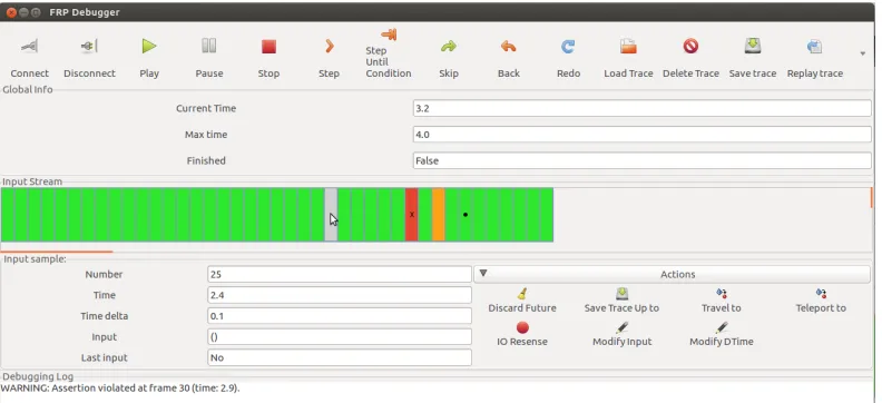
Fig. 4. Screenshot of our FRP game debugger, with the central area showing a loaded input stream being used to execute a game on a mobile phone. The screenshot shows a sample in which a temporal assertion was violated (red), the current sample according to the phone (orange), a breakpoint (dot), and the sample selected by the user (grey).

violated. As the phone follows the debugging GUI as it moves along the trace, it will actually show the animation going backwards, forwards and jumping steps as instructed, which is an excellent visual aid for developers. Furthermore developers can hot-swap the game, that is, make changes to the program, recompile it, restart it on the phone, and take it back to the same point in time to see if the bugs persist, all without having to close the GUI application.

Second, and aided by this first feature, we can take the user traces and feed them to QuickCheck in order to find bugs. The Stream Manipulation API presented in Section 5 allows us to instruct QuickCheck to take part of an input stream from a real user and continue it randomly to try and find counter-examples for the game properties. As QuickCheck generates new input traces as counter-examples, we can save them in files, load them in the debugger and on the phone, and visualize the issue. So, in effect, we can see QuickCheck play.

As an example, let us show how we can use this approach to debug the input stream provided by QuickCheck invalidating the propertypropTestBallOverFloor(Section 5). If we connect an Android phone running this application with our debugger, we can use the GUI to load the counter-example input stream generated by QuickCheck and visualize on the phone the point at which our assertion fails (Figure 5):

The fact that we can rely on Haskell’s purity and explicit, strong types to obtain the referential transparency needed to debug deterministically supports the idea that pure Functional Programming is a very good fit for developing many kinds of games.

7 EXPERIENCE

(a) Frame #1: 0s. (b) Frame #3: 5.5176s. (c) Frame #4: 8.5218s. (d) Frame #5: 9.5218s.

Fig. 5. Screenshots of the game running on an Android phone being remotely controlled using our FRP debugging GUI, executing the counter-example generated by QuickCheck, step-by-step. The ball is under the floor after 2 frames and takes 2 more frames to come back to the screen area. Frames #3 and #4 produce assertion violations while the ball is below the floor.

The combination of Temporal Logic, QuickCheck and our debugging GUI application has also been used to debug existing demonstration Yampa games like Haskanoid1_{, professional iOS/Android}

games like Magic Cookies!2,3and other titles currently under development4.

Fig. 6. Screenshot of the Yampa game Haskanoid running on an Android tablet.

1_{http://github.com/ivanperez-keera/haskanoid}

2_{https://itunes.apple.com/us/app/magic-cookies/id1244709871}

3_{https://play.google.com/store/apps/details?id=uk.co.keera.games.magiccookies}

4_{The development of the mobile extensions to the framework presented in this paper and their use to test these games}

7.1 Haskanoid

To demonstrate properties that QuickCheck can detect and how it has helped find bugs in games, we provide examples using the existing game Haskanoid (Figure 6), a Haskell implementation of Arkanoid that runs on Windows, Linux, Mac, iOS, Android and can be controlled with devices like Kinects, Wiimotes and accelerometers.

The player controls a paddle which moves only sideways. A ball is initially attached to the paddle. When the user clicks the mouse, the ball is propelled upwards, bouncing against walls, blocks and the paddle itself. Blocks disappear when hit three times. The player wins when all blocks disappear, and loses if the ball hits the floor.

The full game implements more complex features like levels, lives and sound. Here we present a simplified version to test the game physics and simple, yet important, game invariants.

7.1.1 Objects.Objects in Haskanoid are defined as signal functions that, depending on some input, present their new state and any effects that could affect other objects or their own existence (i.e. requests to create new objects or kill themselves). This idea is described in more detail in [Courtney et al. 2003].

typeObjectSF=SF ObjectInput ObjectOutput

dataObjectInput=ObjectInput

{userInput ::Controller ,collisions ::Collisions ,knownObjects::Objects

}

dataObjectOutput=ObjectOutput

{outputObject ::Object ,harakiri ::Event()

}

Any game object can depend on the user input (Controller), previous collisions, and the state of other objects. Game objects produce an internal state with physical properties and indicate whether the object has died. This is used by blocks hit by the ball, to signal that they must be eliminated.

A simplified definition for objects, used for for the ball, the paddle, blocks and the walls, follows. All 2D-suffixed types correspond to tuples ofDoubles.

dataObject=Object

{objectName ::String ,objectKind ::ObjectKind ,objectPos ::Pos2D ,objectVel ::Vel2D ,objectAcc ::Acc2D ,objectHit ::Bool ,objectDead ::Bool ,collisionEnergy::Double

}

the ball could overlap with the wall, or pass through blocks exhibiting an effect calledtunnelingor bullet through paper[Gregory 2014].

propBallInScreenAreaW=forAll myStream$evalT Always

(Prop(mainGame≫arr gameObjects≫arr(λp→isInRange(0,gameWidth) (fst(ballPos p)))))

wheremyStream::Gen Controller myStream=uniDistStream >quickCheck propBallInScreenAreaW

∗∗∗Failed!Falsifiable(after31tests):

(Controller {controllerPos=(8.49338899008,29.07069391684),controllerClick=False},

[(17.68729810519,Controller {controllerPos=(28.12964084927,12.4975777242),controllerClick=True}) ,(29.88005602026,Controller {controllerPos=(51.41061779016,3.0186952000), controllerClick=False})])

In this trace, QuickCheck is telling us that the input controller (e.g. mouse) needs to start at a particular position with the main button released, moved to another position with the button pressed, and moved elsewhere with the button released. However, the delays between one sample and the next are unrealistically large: one new frame every 15 seconds. To make it a bit more realistic we decide to use a stream generator that guarantees shorter delays. Let’s assume that our game runs at around 25FPS (denseStreamis an auxiliary generator that creates streams with very small time deltas following a normal distribution):

propBallInScreenAreaW′=forAll myStream$evalT Always

(Prop(mainGame≫arr gameObjects≫arr(λp→isInRange(0,gameWidth) (fst (ballPos p)))))

wheremyStream::Gen Controller myStream=denseStream0.04 >quickCheck propBallInScreenAreaW′ + + +OK,passed100tests◦

If we try this property with even higher framerates (lower deltas), it seems to pass all tests. But that is only an illusion. If, instead of increasing the number of deltas, we choose to increase the number of tests, we start seeing that not even 0.04 is low enough:

>quickCheckWith(stdArgs{maxSuccess=100000})propBallInScreenAreaW′

∗∗∗Failed!Falsifiable(after3443tests):...

There is one artificial way in which we can prevent the ball from going out of the screen: with a speed cap. If we cap the maximum speed and introduce a margin of error in the detection of collisions, then the collision with the ball against any wall will be detected before they overlap.

Nevertheless, this artificial cap can easily be tested for by checking the magnitude of the ball’s velocity. This test should work regardless of the sampling rate and detecting that the ball moves too fast (one condition) is easier than detecting that the ball is out of the screen, because it was moving too fast (two conditions).

propVelInRange=forAll myStream$evalT Always

(Prop(mainGame≫arr gameObjects≫arr(λp→isInRange(0,800) (norm(ballVel p)))))

wheremyStream::Gen Controller myStream=denseStream0.004 >quickCheck propVelInRange

∗∗∗Failed!Falsifiable(after67tests):

(Controller {controllerPos=(130.5942684124,40.2324487584),controllerClick=False},

[(3.9907922435e−3,Controller{controllerPos=(61.5220268505,108.729668432),controllerClick=True}), (2.1598144494e−3,Controller{controllerPos=(66.5487565898,50.682566812), controllerClick=False})])

In this trace, the mouse is moved quickly to the left and clicked, propelling the ball with a velocity of thousands of pixels per second. By adding the cap in other places in the code, we guarantee that the velocity is within the expected range, making the ball more likely to remain within the game area even with lower sampling rates. This solution is, unfortunately, ad hoc and not reusable, and it might not behave properly in other situations. A general solution for this problem, calledtunneling, is to implement a continuous-collision detection system (CCD).

8 RELATED WORK

The link between FRP and Temporal Logic has been studied extensively. Jeffrey [2012] describes how LTL can be used to encode FRP’s construct types, making any well-typed FRP program a proof of an LTL tautology. Jeffrey [2014] also combines LTL with FRP using dependent types to define streams of types, which themselves type reactive programs and form a constructive temporal logic, exploiting the Curry-Howard isomorphism between TL and FRP. The author goes on to define a combination of FRP with past-time LTL, in which combinators like “always” mean “so far”, making all modalities executable and causal.

Jeltsch [2012] has also described the Curry-Horward isomorphism between Temporal Logic and FRP, in which FRP programs implement Temporal Logic propositions. The author shows that behaviours and events can be generalized in terms of the Until operator from LTL [Jeltsch 2013]. He then gives categorical semantics for LTL with until and FRP with behaviours and events. This work is used to define Concrete Process Categories (CPCs), which serve as categorical models of FRP with processes. The author defines a new semantics, a new temporal logic for CPCs, which captures causality.

Sculthorpe [2011] has described an encoding of Priorean Temporal Logic in a denotational model used to describe FRP signals. In his approach, properties of both the time domain and FRP signals and signal functions can be described as temporal predicates, that may or may not hold, depending on the time domain. Sculthorpe also shows how properties of signal functions, like being temporally decoupled or stateless may be captured using temporal logic. There are several differences between Sculthorpe’s approach and ours. First, we use a different kind of time, which is bounded because our simulations can actually end. Also, because we are interested in executing or checking these properties live, we cannot depend on the past or the future in the way that Sculthorpe’s semantics does. Dependencies on the past lead to leaks, dependencies on the future cannot be determined in the present (which is how Yampa is evaluated).

The use of Temporal Logic to specify properties of reactive systems is frequent in other domains. Hughes et al. [2010] use Temporal Logic to specify parts of an asynchronous messaging server, and use QuickCheck to prove properties under timing uncertainty. Tan et al. [2004] provide a metric to understand how well a property specified using Temporal Logic has been tested by a test suite.

Giannakopoulou and Havelund [2001] presents an approach at verifying a program’s behaviour against LTL specifications, by translating an LTL formulae into a finite-state automata that monitors the program’s behaviour. This approach is based on the next-free variant of Linear Temporal Logic with Until, as it is guaranteed to be unaffected bystuttering(receiving the same input several times in succession).

Havelund and Rosu [2001] have also used Linear Temporal Logic to monitor programs by connecting to them running live via the network. In this work the authors use finite-trace LTL, a variant of infinite-trace LTL in which always means at every pointin the trace, and next defaults to true at the end of the trace. Some formulae that always hold in limited-trace LTL do not hold in infinite-trace LTL and vice-versa, an aspect explored in also in some detail by Sculthorpe [2011]. The use of this logic also results in counter-intuitive properties, for example, at the end of the trace, bothnext Xandnext(neg X)hold for anyX.

Nejati et al. [2005] discuss the construction of a model that approximates a program of interest, and use CTL to verify properties of the model. The authors use a three-valued logic in order to indicate when a model needs further refinements and determine whether a CTL property holds.

In the context of game programming, the idea of recording and replaying programs determinis-tically was proposed, among others, by John Carmack [Carmack 1998, p. 55], who implemented a single entry point for all input events to a game, and set up a journaling system that recorded everything the game received, including the time. Carmack also pointed out that reproducing bugs is key to fixing them, and that it is important to be able to roll back time in order to find when a bug is first introduced, even if its effect is only visible later in the execution.

Execution-replay systems have also been studied in the context of general imperative program-ming and especially parallel and distributed systems [Cornelis et al. 2003; Ronsse et al. 2000]. Much of the focus in those areas has been towards dealing with low-level issues to guarantee determinism of replays. In contrast, we rely on Haskell’s strong type system to guarantee the freedom from side effects in FRP programs and hence absolute determinism, letting us focus on how to exploit such guarantees for declarative testing and debugging. Our debugger currently records complete input traces, but our approach could be used to log input to only a subpart of the system, making it more suitable for higher-level debugging, as opposed to logging low-level system calls.

Mozilla’s toolrr5_{monitors a group of Linux processes, capturing the results of kernel calls and}

non-deterministic CPU effects. In future replays, memory and register contents are the same, and all system calls return the same values. This tool has been designed for general purpose applications, so it works at a very low level. As a result, it is tied to the Linux kernel, it emulates a single-core machine, and it is difficult to port to other architectures (ARM and Android support, for example, is still an open issue6). In contrast, our approach works on all architectures for which there is a Haskell Compiler with a corresponding back-end (currently iOS, Android, web, Linux, Windows and MacOSX). To control a simulation with the debugging GUI, the only platform-specific adaptation required is a way for the Yampa debugger to open two network sockets for communication.

GDB hasProcess Record and Replay7, capabilities, which record system calls and the CPU and memory state at each point. Like Mozilla’s rr, GDB’s replay feature requires adaptations specific

5_{http://rr-project.org/}

for each architecture and system call. An advantage of GDB’s implementation is that actions are undoable, which means that we can move backwards along the trace. In contrast, FRP signals only move forward, although our system records intermediate Signal Functions to provide random access to any time point in constant time, and they can always be reproduced deterministically if only the inputs are recorded. Time-reversible FRP combinators remain an open problem.

9 CONCLUSIONS AND FUTURE WORK

In this paper we have shown how to approach testing and debugging of FRP programs in variants like Arrowized FRP that completely separate IO from the signal processing. We have used an encoding of Linear Temporal Logic over FRP to describe temporal properties of FRP programs and evaluate them against input streams. We have also shown that this simple approach makes FRP programs easily testable with existing tools like QuickCheck, and we can add temporal assertions to programs in a similar fashion.

We have extended an FRP implementation with recording and remote control capabilities, and implemented a Graphical User Interface to communicate with games running remotely on PCs, iOS devices and Android phones. The referential transparency available in pure FRP implementations like Yampa helps developers reproduce the exact same situation witnessed by beta-testers, and move back and forth along the trace adding new assertions or visualizing the simulation along on a phone to pinpoint possible bugs. These traces can be fed to QuickCheck for additional help in finding possible property violations, and the counter-examples found by QuickCheck can be loaded back into a phone for future study and to visualize them. So, in practice, we can truly see QuickCheck play our games.

We would also be interested in finding games for which the temporal language provided is insufficient to express desired properties declaratively and concisely. Our encoding of temporal properties is based on Linear Temporal Logic, but we can answer questions pertaining to multiple possible futures by means of the quantification provided by QuickCheck withforAlland the stream generators we provide. Nevertheless, the use of a different formalism like Computation Tree Logic and a comparison with our approach remain as future work.

A question we have not answered is how well the input space is explored. In this respect, further improvements could be made by adding Signal Function generators, increasing the confidence on abstract properties about Signal Functions, like the Arrow laws that they are expected to fulfill. We have also yet to explore further shrinking strategies for input traces, in order to help QuickCheck find minimal counter-examples.

Our FRP debugger has been implemented for Yampa, but the same approach could be used with different Arrowized FRP variants like Dunai [Perez et al. 2016]. An advantage of using Dunai over Yampa would be that the former only has one type for Monadic Stream Functions, reducing code duplication in our debugger. Also, Dunai introduces monads, which can be used to implement safe debugging facilities, as shown in Section 6. Additionally, a monad would allow us to introduce the recording system inside a Signal Function, instead of at the top-level like we do in Yampa. This would let us record high-level input, like declarative game actions, instead of low-level input, like user clicks and mouse movement, which would be more useful as small variations to the User Interface are more likely to invalidate the latter.

In some cases we have reduced the debugging facilities introduced in a binary to only saving the inputs to a file, to minimize the overhead and hence the possibility of introducing heisenbugs. If a bug is detected with this minimal debugger and the input is logged accordingly, then it will be completely reproducible with the full debugger.

A side feature facilitated by our framework is that we could stream input traces over to another machine to visualize a game as it is being played, or use them to replay a game in a machine with higher visual specifications or to record a video. We could also replay these games later on in higher quality or record videos of the output for publication online, even if they were produced in devices with lower specifications.

ACKNOWLEDGMENTS

The authors would like to thank P. Capriotti, G. Hutton, J. Bracker, J. Thaler, C. Hruska and the anonymous referees for their constructive comments and helpful suggestions.

REFERENCES

John Carmack. 1998. John Carmack Archive - .plan. http://fd.fabiensanglard.net/doom3/pdfs/johnc-plan_1998.pdf. (1998). Koen Claessen and John Hughes. 2000. QuickCheck: A Lightweight Tool for Random Testing of Haskell Programs. In

Proceedings of the Fifth ACM SIGPLAN International Conference on Functional Programming (ICFP ’00). ACM, New York, NY, USA, 268–279. https://doi.org/10.1145/351240.351266

F. Cornelis, Andy Georges, M. Christiaens, Michiel Ronsse, T. Ghesquiere, and K. De Bosschere. 2003. A taxonomy of execution replay systems.Proceedings of International Conference on Advances in Infrastructure for Electronic Business, Education, Science, Medicine, and Mobile Technologies on the Internet(2003).

Antony Courtney, Henrik Nilsson, and John Peterson. 2003. The Yampa Arcade. InProceedings of the 2003 ACM SIGPLAN Workshop on Haskell (Haskell ’03). ACM, New York, NY, USA, 7–18. https://doi.org/10.1145/871895.871897

Conal Elliott and Paul Hudak. 1997. Functional Reactive Animation. InInternational Conference on Functional Programming. 163–173.

E. Allen Emerson. 1990. Handbook of Theoretical Computer Science (Vol. B). MIT Press, Cambridge, MA, USA, Chapter Temporal and Modal Logic, 995–1072. http://dl.acm.org/citation.cfm?id=114891.114907

D. Giannakopoulou and K. Havelund. 2001. Automata-based verification of temporal properties on running programs. InProceedings 16th Annual International Conference on Automated Software Engineering (ASE 2001). 412–416. https: //doi.org/10.1109/ASE.2001.989841

Jim Gray. 1986. Why Do Computers Stop and What Can Be Done About It?. InSymposium on Reliability in Distributed Software and Database Systems. 3–12. http://citeseerx.ist.psu.edu/viewdoc/summary?doi=10.1.1.59.6561

Jason Gregory. 2014.Game Engine Architecture, Second Edition(2nd ed.). A. K. Peters, Ltd., Natick, MA, USA.

Klaus Havelund and Grigore Rosu. 2001. Monitoring programs using rewriting. InAutomated Software Engineering, 2001.(ASE 2001). Proceedings. 16th Annual International Conference on. IEEE, 135–143.

John Hughes. 2000a. Generalising monads to arrows.Science of computer programming37, 1 (2000), 67–111. John Hughes. 2000b. Generalising monads to arrows.Science of computer programming37, 1 (2000), 67–111.

John Hughes, Ulf Norell, and Jérôme Sautret. 2010. Using temporal relations to specify and test an instant messaging server. InThe 5th Workshop on Automation of Software Test, AST 2010, May 3-4, 2010, Cape Town, South Africa. 95–102. https://doi.org/10.1145/1808266.1808281

Alan Jeffrey. 2012. LTL Types FRP: Linear-time Temporal Logic Propositions As Types, Proofs As Functional Reactive Programs. InProceedings of the Sixth Workshop on Programming Languages Meets Program Verification (PLPV ’12). ACM, New York, NY, USA, 49–60. https://doi.org/10.1145/2103776.2103783

Alan Jeffrey. 2014. Functional Reactive Types. InProceedings of the Joint Meeting of the Twenty-Third EACSL Annual Conference on Computer Science Logic (CSL) and the Twenty-Ninth Annual ACM/IEEE Symposium on Logic in Computer Science (LICS) (CSL-LICS ’14). ACM, New York, NY, USA, Article 54, 9 pages. https://doi.org/10.1145/2603088.2603106 Wolfgang Jeltsch. 2012. Towards a Common Categorical Semantics for Linear-Time Temporal Logic and Functional Reactive

Programming.Electron. Notes Theor. Comput. Sci.286 (Sept. 2012), 229–242. https://doi.org/10.1016/j.entcs.2012.08.015 Wolfgang Jeltsch. 2013. Temporal Logic with "Until", Functional Reactive Programming with Processes, and Concrete

Process Categories. InProceedings of the 7th Workshop on Programming Languages Meets Program Verification (PLPV ’13). ACM, New York, NY, USA, 69–78. https://doi.org/10.1145/2428116.2428128

Chris Lewis, Jim Whitehead, and Noah Wardrip-Fruin. 2010. What Went Wrong: A Taxonomy of Video Game Bugs. In

108–115. https://doi.org/10.1145/1822348.1822363

Shiva Nejati, Arie Gurfinkel, and Marsha Chechik. 2005. Stuttering abstraction for model checking. InSoftware Engineering and Formal Methods, 2005. SEFM 2005. Third IEEE International Conference on. IEEE, 311–320.

Henrik Nilsson, Antony Courtney, and John Peterson. 2002. Functional Reactive Programming, Continued. InProceedings of the 2002 ACM SIGPLAN workshop on Haskell. ACM, 51–64.

Gergely Patai. 2009. Eventless reactivity from scratch.Draft Proceedings of Implementation and Application of Functional Languages (IFL’09)(2009), 126–140.

Ross Paterson. 2001. A new notation for arrows.ACM SIGPLAN Notices36, 10 (2001), 229–240.

Ivan Perez, Manuel Bärenz, and Henrik Nilsson. 2016. Functional Reactive Programming, Refactored. InProceedings of the 9th International Symposium on Haskell (Haskell 2016). ACM, New York, NY, USA, 33–44. https://doi.org/10.1145/2976002. 2976010

Ivan Perez and Henrik Nilsson. 2015. Bridging the GUI Gap with Reactive Values and Relations. InProceedings of the 2015 ACM SIGPLAN Symposium on Haskell (Haskell ’15). ACM, New York, NY, USA, 47–58. https://doi.org/10.1145/2804302.2804316 Amir Pnueli. 1977. The temporal logic of programs. InFoundations of Computer Science, 1977., 18th Annual Symposium on.

IEEE, 46–57.

Arthur N Prior. 1967.Past, present and future. Vol. 154. Oxford University Press.

Michiel Ronsse, Koen De Bosschere, and Jacques Chassin De Kergommeaux. 2000. Execution replay and debugging.arXiv preprint cs/0011006(2000).

Neil Sculthorpe. 2011. Towards safe and efficient functional reactive programming. Ph.D. Dissertation. University of Nottingham.

Li Tan, Oleg Sokolsky, and Insup Lee. 2004. Specification-based testing with linear temporal logic. InInformation Reuse and Integration, 2004. IRI 2004. Proceedings of the 2004 IEEE International Conference on. IEEE, 493–498.

J. A. Whittaker. 2000. What is software testing? And why is it so hard? IEEE Software17, 1 (Jan 2000), 70–79. https: //doi.org/10.1109/52.819971