Type 2 fuzzy alpha cuts

Type-2 Fuzzy Alpha-cuts

Hussam Hamrawi

College of Computer Sciences University of Bahri

Khartoum, Sudan Email: hussamw@bahri.edu.sd

Simon Coupland

Centre for Computational Intelligence De Montfort University

Leicester, UK Email: simonc@dmu.ac.uk

Robert John

Automated Scheduling Optimisation and Planning School of Computer Science

University of Nottingham Nottingham, UK

Email: robert.john@nottingham.ac.uk

Type-2 fuzzy logic systems make use of type-2 fuzzy sets. To be able to deliver useful type-2 fuzzy logic applications we need to be able to perform meaningful operations on these sets. These operations should also be practically tractable. However, type-2 fuzzy sets suffer the shortcoming of being complex by definition. Indeed, the third dimension, which is the source of extra parameters, is in itself the origin of extra computational cost. The quest for a representation that allow practical systems to be implemented is the motivation for our work. In this paper we define the alpha-cut decomposition theorem for type-2 fuzzy sets which is a new representation analogous to the alpha-cut representation of type-1 fuzzy sets and the extension principle. We show that this new decomposition theorem forms a methodology for extending mathematical concepts from crisp sets to type-2 fuzzy sets directly. In the process of developing this theory we also define a generalisation that allows us to extend operations from interval type-2 fuzzy sets or interval valued fuzzy sets to type-2 fuzzy sets. These results will allow for the more applications of type-2 fuzzy sets by expiating the parallelism that the research here affords.

I. INTRODUCTION

Zadeh [33]–[35] defined the type-2 fuzzy set (T2FS) along with a plethora of concepts and mathematical func-tions including the extension principle (EP) and resolution identity more commonly known as theα-cut decomposition theorem. The EP extends point-valued operations from the crisp mathematical setting to a corresponding fuzzy mathe-matical setting, essentially fuzzifying classical mathemathe-matical concepts. Theα-cut decomposition theorem also allows the same extension to be performed in a set-valued manner. The idea is to decompose fuzzy sets into a collection of crisp sets related together via theαlevels. This decomposition theorem has been extended to fuzzy sets with interval membership grades known either by interval valued fuzzy sets (IVFSs) or interval T2FSs (IT2FSs) [20]. Type-2 fuzzy sets, (both general and interval), have attracted much attention amongst researchers both in theory and applications (e.g. [3], [5], [8], [13], [14], [24], [25], [28], [29]) mainly for the extra dimension they exhibit, which gives these sets the potential to model extra uncertainty based information. To be able to make use of T2FSs, we should be able to perform meaningful operations on these sets and these operations should also be practically tractable. T2FSs suffer the shortcoming of being complex by definition. Indeed, the third dimension, which

is the source of extra parameters, is in itself the origin of extra computational cost. The quest for a representation that allow practical systems to be implemented is a fertile field of research. There are four main representation theorems for T2FSs, in which practical applications and theoretical defi-nition have been investigated. The vertical slice, wavy slice [22], alpha-plane (or zSlices) [17], [27] and geometric [5] representations. Zadeh [33] was the first to define operations for T2FSs, utilisingα-cuts of each fuzzy membership grade. Recently, Chen and Kawase [4], Tahayori et al. [26], Liu et al. [17], [19], and Wagner and Hagras [27], [28] focused their attention towards decomposing T2FSs into several IVFSs. In particular, Liu [17] defined α-planes and Wagner and Hagras [27] defined zSlices as part of their effort to calculate the Centroid of T2FSs. In his work, Liu concluded that the union, intersection and centroid of T2FSs is equal to their respective operations of its constituent α-planes. Wagner and Hagras independently concluded the same. Hamrawi and Coupland [9], [10] derived arithmetic operations and defined non-specificity for T2FSs using the same concept and stated a generalised formula in [11], [12]. In this paper we investigate the use of the concept of α-cuts and its extension principle for T2FSs. We explain, step by step, the development phases of the theory and definitions. We believe it is a significant step forward in the theory and application of T2FSs. The novel ideas provided in this paper, are themselves built upon existing theories and definitions well accepted in the literature and is an extension to available and definitions. We show how operations on general type-2 fuzzy sets can be broken down into a collection of interval type-2 or crisp interval operations. The paper is organised as follows: Section 2 provides the notations and necessary back ground for the following work; Section 3 revisits theα -plane representation and defines theα-plane extension prin-ciple; Section 4 discusses theα-cut representation of IVFSs; Section 5 defines the α-cut representation for T2FSs and the extension principle associated with this representation; Section 6 provides a conclusion.

II. DEFINITIONS

A. Basic Definitions

X, it is a functionA:X → {0,1}that assigns1to elements of the domain that belong to A and 0 otherwise. Let C(X) be the set of all crisp subsets ofX 1_{. LetAbe an Interval} over X. It is defined by A = [x, x] where x, x ∈ X and x≤x. Also let I(X) be the set of all interval subsets of X. Note that an interval is a special crisp set with A(x) = 1, x≤x≤xand0otherwise. Let a type-1 fuzzy set (T1FS)A be a subset ofX, and defined to be a functionA:X→[0,1]. It is a generalisation of both crisp sets and intervals. We call a T1FS, a fuzzy set (FS) for short. Let F(X) be the set of all fuzzy subsets of X, and all FSs defined in this paper be convex. In this paper we are particularly interested in the α-cut representation of FSs. The α-cut of FS, Aon the domainX, is a crisp set defined to beAα={x|A(x)≥α},

α∈ [0,1],x ∈X. Eachα-cut is associated with a special FS, αAα ∈ F(X), and called α-FS. It is defined such that

αAα(x) =α∧Aα(x),∀x[16], [23], [32]. Then the α-cut representation theorem (α-RT) [16] is defined to be the union of all such α-FSs, i.e., A=S

∀ααAα. It is evident that the membership grade of each domain value,x, can be calculated by A(x) = sup∀ααAα(x). If the FS, A, is continuous then its α-cut is an interval, Aα ∈ I(X), which can be written

Aα = [xα, xα]. The strong α-cut is another useful crisp set defined to beAα+ ={x|A(x)> α} [16]. In order to define operations for FSs, Zadeh defined the extension principle (EP), in which a function is extended from crisp sets to FSs in a compositional relation between point-values. This EP is sometimes referred to as thesup−mincomposition. Let, X =X1×...×Xn, be the Cartesian product of universes, and A1, ..., An be FSs in each universe respectively. Also

let Y be another universe and B ∈ Y be a FS such that

B = f(A1, ..., An), where f : X → Y. Then the EP is defined as follows [33]:

B⇔B(y) = sup

(x1,...,xn)∈f−1(y)

min (A1(x1), ..., An(xn))

(1) where f−1_{(y) is the inverse function of y =f(x}

1, ..., xn).

Zadeh also defined the α-cut version of the EP (α-EP) to

extend operations from crisp sets to FSs directly in a set-valued method. It is defined as follows [33]2_:

B=f(A1, ..., An) =

[

∀α

αf(A1α, ..., Anα) (2)

Some researchers have asserted that equations (1) and (2) are equal [1], [23], [33]. An interval valued fuzzy set (IVFS),

ˆ

A, over X is defined by a function Aˆ : X → I([0,1]), then Aˆ(x) = [u_x, ux] and we let, Fˆ(X), be the set of all

IVFSs on X. The upper membership function (UMF) of

an IVFS, Aˆ, is a fuzzy set, A, where A(x) = ux, ∀x. The lower membership function (LMF) of an IVFS, Aˆ, is a fuzzy set, A, where A(x) =ux, ∀x. We can see that an IVFS is completely determined by the LMF and UMF, i.e.,

1_{This is the powerset in classical set theory. We use a different notation to}

allow us to easily distinguish between the powerset of crisp value, intervals and fuzzy sets.

2_{Throughout this paper we use}S_{to denote both crisp and fuzzy union.}

When used in a fuzzy union we are referring to the maximum t-conorm. ˆ

A = A, A

which means Aˆ(x) =

A(x), A(x)

, ∀x. Let, X =X1×...×Xn, be the Cartesian product of universes, andAˆ1, ...,Aˆn be IVFSs in each universe respectively. Also

let Y be another universe and Bˆ ∈ Y be an IVFS such

that Bˆ =f( ˆA1, ...,Aˆn), wheref :X →Y is a monotonic

mapping. Then to use the Extension Principle with IVFSs, the (IVEP) can be defined as follows:

ˆ

B≡ B, B

= f(A1, ..., An), f(A1, ..., An)

(3)

This means, to derive operations for IVFSs we only need to derive operations for their upper and lower membership functions3_.

B. Type-2 Fuzzy Set Definitions

In this section we review the main definitions of T2FSs.

Let A˜ be a T2FS in the universe X. It is a function

˜

A:X →F([0,1]), so the membership grade of each domain value of the T2FS is a FS defined on the unit interval, i.e., A˜(x) ∈ F([0,1]). The vertical slice (VS) [18], [22], i.e., A˜x ≡ A˜(x) is a FS with domain values ux ∈ [0,1] called the primary grades (PGs) and membership grades

˜

Ax(ux) ∈ [0,1] called the secondary grades (SGs). Each PG is associated with one SG and the union of all the primary grades ux of domain value xis called the primary membership (PM), i.e., Jx = u1x, u2x, ..., uq x if the domain of membership grades of the T2FS is discrete, and Jx= [ux, ux]if it is continuous. Normally, it is assumed that the PMs are intervals, and in the discrete case the PM can be calculated by considering the lower and upper bounds, i.e., Jx =

infi=1,...,quix,supi=1,...,quix

, and henceJx∈ I([0,1]). The union of all primary memberships is called the footprint of uncertainty (FOU),F OU( ˜A) =S

∀x(x, Jx). A T2FS can be represented by the union of all its VSs which is called the vertical slice representation, i.e.,

˜

A=[

∀x

x,A˜x

(4)

An interval type-2 fuzzy set (IT2FS) is a T2FS where all the secondary grades are at unity, i.e., A˜x(ux) = 1, ∀ux∈

Jx, ∀x ∈ X. It is well known that an IT2FS can be

completely determined using its F OU and it is the same as an IVFS [2], [21]. Recently, Liu [17] proposed the α -plane representation of T2FSs, and Wagner and Hagras [27] proposed zSlices. Liu defined an α-plane,A˜α˜ 4, of a T2FS,

˜

A, to be the union of the PGs of A˜, whose SGs are greater than or equal to levelα˜, i.e.,

˜

Aα˜=

n

(x, ux)|A˜x(ux)≥α,˜ ∀x, ∀ux∈Jx o

(5)

Then Liu defines an indicator function,I_A˜_α˜, acting onx∈X

such that,

I_A˜_α˜(x, ux) =

1, (x, ux)∈A˜α˜

0, (x, ux)∈/A˜α˜

(6)

Then a T2FS associated with each α-plane,α˜A˜α˜, is defined

as follows:

˜

αA˜α˜= (x, ux),α˜·I_A˜_α˜(x, ux)|∀x∈X (7)

Using this definition the T2FS,A˜, is represented by the union of all its associated T2FSs, i.e.,

˜

A=[

∀α˜

˜

αA˜α˜ (8)

Note that we do not use an indicator function to defineα-cuts for FSs, and hence we will provide a different interpretation to that of Liu in Section III of this paper. We define the α-plane RT in an analogous way to that of the α-cut RT for FSs. The EP for T2FSs (T2EP) is defined in a similar way to the FS EP [18]. Let, X = X1×...×Xn, be the Cartesian product of universes, and A˜1, ...,A˜n be T2FSs in each universe respectively. Also let Y be another universe andB˜ ∈Y be a T2FS such thatB˜ =f( ˜A1, ...,A˜n), where

f :X →Y is a monotone mapping. Then applying the EP

to T2FSs (T2EP) lead to the following:

˜

B ⇔B˜(y) = sup

(x1,...,xn)∈f−1(y)

minA˜1(x1), ...,A˜n(xn)

(9) where y = f(x1, ..., xn), and A˜1(x1), ...,A˜n(xn) are the

VSs which can be written as A˜1x1, ..., ˜

Anxn. These defini-tions are used to formulate theα-cut representation theorem for T2FSs.

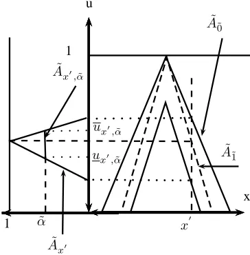
1 u

x ˜

A˜₀

˜

A˜1

x′

˜

A_x′

1 α˜

˜

A_x′_,α˜

ux′_,α˜

u_x′_,α˜

Fig. 1. 2D representation of the T2FS with triangular vertical slices.

III. T2FS ALPHA-PLANEEXTENSIONPRINCIPLE

In this section we introduce a generalisation that allows us to extend operations from IVFSs to T2FSs directly using α-planes. This theory lays the foundation for the α-cut decomposition theorem for T2FSs. This method has been stated without a proof by Hamrawi and Coupland [10], with a proof being provided in Hamrawi et al. [11], [12]. Here we start with a discussion on α-planes, and the α-plane

1 u

x

0 1 2 3 4

α3

α2

α1

A

A

L_x

αLxα RxαRxα

Fig. 2. Continuous IVFSAˆand itsα-cuts

representation theorem (RT). We investigate some of the properties of these α-planes and then define the α-plane extension principle (α-PEP).

A. α-planes Revisited

First, the steps Zadeh [33] took in order to define the intersection of two T2FSs are summarised in two stages:

1) Extend the FS definition to fuzzy sets with interval-valued membership functions.

2) Generalise from intervals to fuzzy sets by the use of theα-cut form of the EP (α-EP).

In the sequel, we follow these steps in order to decompose T2FSs into its elementary components, i.e. crisp sets. In general, since each VS is a FS, then it can be decomposed using theα-cut decomposition theorem. LetA˜∈F˜(X) be a T2FS onX, whereA˜xis its VS atx. Theα-cuts of each VS are A˜x,α˜=

n

ux|A˜x(ux)≥α˜ o

,∀ux∈Jx. If the domain of the T2FS membership function is assumed to be continuous thenA˜x,α˜=

ux,α˜, ux,α˜

. Since these VSs are FSs then they can be represented by theα-cut decomposition theorem, i.e.,

˜

Ax= [

∀α˜

˜

αA˜x,α˜ (10)

where α˜A˜x,α˜ is the special FS (α-FS) associated with each

α-cut. It is defined as α˜A˜x,α(˜ ux) = ˜α∧ A˜x,α(˜ ux) and

˜

Ax,α(˜ ux) = 1ifux∈A˜x,α˜ and zero otherwise. Then, T2FS

˜

A is the union of all its VSs, therefore,

˜

A=[

∀x

x,[ ∀α˜

˜

αA˜x,α˜

!

(11)

This is a very important result as a T2FS is represented using a collection of crisp sets (or intervals) defined vertically. Now let us take the union of all theα-cuts across all domain values for only one level, i.e.,S

∀x

x,A˜x,α˜

. It is the union of all

same as theα-plane definition of equation (5).

˜

Aα˜ =

[

∀x

x,A˜x,α˜

=n(x, ux)|A˜x(ux)≥α,˜ ∀x, ∀ux∈Jx o

(12)

Here it is clear that

˜

Aα(˜ x, ux) = ˜Ax,α(˜ ux)

We turn our attention to the α-FSs of each VS. Let us

take the union of all the α-FSs across all domain values for only one level, i.e.,S

∀x

x,α˜A˜x,α˜

. It is a T2FS with

membership grades α˜A˜x,α˜, which are FSs themselves, i.e.,

˜

αA˜x,α˜ =S∀ux

ux,α˜A˜x,α(˜ ux)

. This is exactly the same as the T2FS associated with eachα-plane defined in equation (7).

˜

αA˜α˜ =

[

∀x

x,α˜A˜x,α˜

= ˜α[ ∀x

x,A˜x,α˜

=n(x, ux),α˜A˜α(˜ x, ux)

|∀x∈Xo

(13)

We call this special T2FS associated with eachα-plane, (α -T2FS), following the same convention we used for FSs. we

note that this same definition is called,α-FOU in [19], and zSlice in [27]. We can see that a T2FS is decomposed of theseα-T2FSs.

Theorem 3.1 (α-Plane RT): A type-2 fuzzy set,A˜, can be represented (decomposed) of the union of all its α-T2FSs, i.e.,

˜

A=[

∀α˜

˜

αA˜α˜ (14)

Proof. Straight forward from equations (11).(12) and (13).

In most cases the α-plane,A˜α˜, is considered to be an IVFS

or an IT2FS [17], [19], [27], [28]. This is only the case when the VSs are continuous functions and hence Jx∈I([0,1]) is an interval. If the VSs are in discrete domains then as men-tioned earlier, the PMs must be bounded through a bounding operation. The following worked example demonstrates how to construct IVFS α-planes for discrete T2FSs.

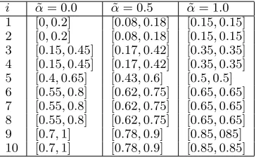
Example 3.1: Let X = {xi|i= 1,2, ...,10}, and

very small(V S), small(S), medium(M), large(L), and very large(V L) ∈ F([0,1]) are the FSs that represent the vertical slices, A˜x, defined in Table I. Each vertical slice, A˜xi, consist of PGs, uxi, forming its domain and the SGs,A˜xi(uxi), forming its membership grade. Let also,

˜

A ∈ F˜(X), be defined as in Table II, with domain values,

xi, corresponding to vertical slices from Table I. Table III shows how to extract theα-cuts (α˜) of the VSA˜xi of each domain value to form the crisp sets A˜xi,α˜. Table IV shows

how to construct the interval membership grades of the α -planes,A˜α(˜ xi) =

h

minA˜xi,α˜

,maxA˜xi,α˜

i

in order to formulate the IVFS α-planes.

This example demonstrates the case when there are no gaps in the PM, i.e., all VSs are convex. If there is a contrary case, then these sets are approximated to an IVFS using a bounding operation such as taking the minimum and maximum (or infimum and supremum) of the PGs. Note that if these sets are approximated they risk the loss of information. On the other hand, some might argue, what kind of information do such sets hold? In fact most of the reported applications use a structured model of T2FSs that does not involve such sets.

B. T2FSα-plane EP

In this subsection we formulate a theorem that acts as the α-based EP for T2FSs. It extends operations from IVFSs to T2FSs, directly. We extend these operations using theα -plane RT investigated in the last subsection. Here we state the theorem from Hamrawi et al. [9]–[12].

Theorem 3.2 (α-EP): Let, X = X1×...×Xn, be the Cartesian product of universes, and A˜1, ...,A˜n be T2FSs in each universe respectively. Also let Y be another universe andB˜ ∈Y be a T2FS such thatB˜ =f( ˜A1, ...,A˜n), where

f : X → Y is a monotone mapping. Assume that all the

decomposed α-planes of all the T2FSs (i.e. A˜1, ...,A˜n) are or allowed to be IVFSs. Then B˜ is equal to the union of applying the same function to all the decomposed α-planes of A˜1, ...,A˜n, i.e.,

˜

B =f( ˜A1, ...,A˜n)

=[

∀α˜

˜

αf( ˜A1α˜, ...,A˜nα)˜

(15)

Proof. We start our proof from equation (11)

˜

Ai(x) =[

∀α˜

˜

αA˜ix,α˜

where i= 1, ..., n. Then,

˜

B(y) =f( ˜A1, ...,A˜n)(y)

= sup

(x1,...,xn)=f−1(y)

minA˜1(x1), ...,A˜n(xn)

= sup

(x1,...,xn)=f−1(y)

minA˜1x1, ..., ˜

Anxn

sinceA˜1x₁, ...,A˜nxn ∈F(X) then

˜

B(y) = sup

(x1,...,xn)=f−1(y)

min [

∀α˜

˜

αA˜1x1,α˜, ..., [

∀α˜

˜

αA˜nxn,α˜ !

= sup

(x1,...,xn)=f−1(y) [

∀α˜

˜

αminA˜1x1,α˜, ...,A˜nxn ,α˜

=[

∀α˜

˜

α sup

(x1,...,xn)=f−1(y)

minA˜1x1,α˜, ...,A˜nxn ,α˜

TABLE I

FSS THAT REPRESENT THE VERTICAL SLICES,A˜_x,IN EXAMPLE(3.1). THE HORIZENTAL HEADING REPRESENTS THESGS,A˜_x(u_x),THE VERTICAL HEADING REPRESENTS THEVSS,A˜_x,AND THE NUMBERS IN BETWEEN ARE THEPGS,u_x.

˜

Ax 0.0 0.5 1.0 0.5 0.0

VS 0.0 0.08 0.15 0.18 0.2 S 0.15 0.17 0.35 0.42 0.45 M 0.4 0.43 0.5 0.6 0.65 L 0.55 0.62 0.65 0.75 0.8 VL 0.7 0.78 0.85 0.9 1.0

TABLE II

T2FS,A˜,IN EXAMPLE(3.1). EACH DOMAIN VALUE,x_i,ALONG WITH ITS CORRESPONDING VERTICAL SLICE FROM TABLE(I). xi x1 x2 x3 x4 x5 x6 x7 x8 x9 x10

˜

Axi VS VS S S M L L L VL VL

TABLE III THE CRISP SETα-CUTS,A˜_x

i,α˜,OF THE VERTICAL SLICES,A˜xi,FOR EACH DOMAIN VALUE,xi,IN EXAMPLE(3.1)

i α˜= 0.0 α˜= 0.5 α˜= 1.0 1 0,0.08,0.15,0.18,0.2 0.08,0.15,0.18 0.15 2 0,0.08,0.15,0.18,0.2 0.08,0.15,0.18 0.15 3 0.15,0.17,0.35,0.42,0.45 0.17,0.35,0.42 0.35 4 0.15,0.17,0.35,0.42,0.45 0.17,0.35,0.42 0.35 5 0.4,0.43,0.5,0.6,0.65 0.43,0.5,0.6 0.5 6 0.55,0.62,0.65,0.75,0.8 0.62,0.65,0.75 0.65 7 0.55,0.62,0.65,0.75,0.8 0.62,0.65,0.75 0.65 8 0.55,0.62,0.65,0.75,0.8 0.62,0.65,0.75 0.65 9 0.7,0.78,0.85,0.9,1 0.78,0.85,0.9 0.85 10 0.7,0.78,0.85,0.9,1 0.78,0.85,0.9 0.85

TABLE IV

THE INTERVAL MEMBERSHIP GRADES OF THEα-PLANES,A˜_α˜(xi)IN EXAMPLE(3.1) i α˜= 0.0 α˜= 0.5 α˜= 1.0

1 [0,0.2] [0.08,0.18] [0.15,0.15] 2 [0,0.2] [0.08,0.18] [0.15,0.15] 3 [0.15,0.45] [0.17,0.42] [0.35,0.35] 4 [0.15,0.45] [0.17,0.42] [0.35,0.35] 5 [0.4,0.65] [0.43,0.6] [0.5,0.5] 6 [0.55,0.8] [0.62,0.75] [0.65,0.65] 7 [0.55,0.8] [0.62,0.75] [0.65,0.65] 8 [0.55,0.8] [0.62,0.75] [0.65,0.65] 9 [0.7,1] [0.78,0.9] [0.85,085] 10 [0.7,1] [0.78,0.9] [0.85,0.85]

now we have A˜1α˜, ...,A˜nα˜ ∈Fˆ(X), then we substitute each T2FS with its α-plane representation

f( ˜A1α˜, ...,A˜nα)˜

= sup

(x1,...,xn)=f−1(y)

minA˜1α(˜ x1), ...,A˜nα˜(xn)

then, take the union of all α˜, i.e.,

f( ˜A1α˜, ...,A˜nα)˜

=[

∀α˜

˜

α sup

(x1,...,xn)=f−1(y)

minA˜1α(˜ x1), ...,A˜nα˜(xn) ₍₁₇₎

observe that A˜iα˜(xi) = ˜Ai_xi,α˜, ∀i, it follows that equations (16) and (17) are equal, and that completes the proof. The union, the intersection, and the centroid calculation

IV. ALPHA-CUTS OFINTERVALVALUEDFUZZYSETS

In this section we investigate the α-cuts of IVFSs. We already introduced a method for defining α-cuts of IVFSs in [11], [12] based on earlier work done by Kaufmann and Gupta [15] on fuzzy arithmetic. It is also related to the aggre-gation method defined by Wu and Mendel [30], [31]. Zeng et al. [36], [37] defined a variety ofα-cut RTs for IVFSs and defined the α-EP that makes possible to extend operations from crisp sets to IVFSs directly. Recently, Yager [32] also defined α-cuts and the α-EP for discrete IVFSs. Figueroa Garcia [6], [7] independently introduced alpha-cuts for type-2 interval fuzzy sets, providing an alternative approach to the Karnik-Mendel iterative method for defuzzicafion and for the purposes of formulating and solving linear programming problems. In this section we investigate these methods. We define α-cuts for IVFSs by taking theα-cut of its LMF and UMF which are themselves FSs, i.e.,

Definition 4.1 (IVFSα-cuts): Theα-cut of an IVFS,Aˆ, is defined as follows:

ˆ

Aα= Aα, Aα

where Aˆα(x) =

Aα(x), Aα(x)

.

Note that, the membership of each domain value, x, in the set, Aˆα, is an interval, i.e.,

ˆ

Aα(x) =  



[0,0], x /∈Aα and x /∈Aα [0,1], x /∈A_α and x∈Aα [1,1], x∈Aα and x∈Aα

(18)

These situations are depicted in Figure 3. Notice that we

1 u

x α1

A

A Aα1

Aα1

x1 x2

α2

Aα2

Aα2(x1) = 1

Aα1(x1) =Aα1(x1) = 1

Aα1(x2) = 1

Fig. 3. IVFSAˆ_{, its LMF}A_{, its UMF}A_{and their}α_-cuts.

did not include a particular impossible situation, that of ˆ

Aα(x) = [1,0]. This situation is impossible because, by definition, the LMF is always a subset of the UMF,A⊆A, i.e., A(x) ≤ A(x), ∀x. Which allow us to conclude that A_α ⊆Aα, ∀α. The IVFSα-cuts are pairs that contain two

crisp sets. These sets are treated independently throughout any computation process. This makes it very appealing and holds the semantics of the IVFS definition. The IVFS is actually a FS with an uncertain membership grade which is represented through an interval. The LMF and UMF represents this uncertainty with the interpretation that we do not know exactly the FS, we only know the FS bounds. Again, we follow the same convention of the FSα-cuts and define a special IVFS called (α-IVFS) by defining the special FSs α-FSs for the LMF and the UMF, i.e.,

Definition 4.2 (α-IVFS): A special IVFS (α-IVFS),αAˆα∈ ˆ

F(X), can be defined as follows:

αAˆα= αAα, αAα

=α Aα, Aα

(19)

where αAˆα(x) =

α∧A_α(x), α∧Aα(x)

= α ∧

Aα(x), Aα(x)

.

HereαAˆα is an IVFS, and each domain value,x, is associ-ated with an interval membership grade,αAˆα(x)∈I([0,1]).

Also αA_α and αAα are FSs. The α-cut RT for IVFSs

constitutes the union of all these α-IVFSs.

Theorem 4.1 (IVFS α-cut RT): An interval valued fuzzy set, Aˆ, can be represented by the following α-cut represen-tation theorem:

ˆ

A=[

∀α

αAˆα (20)

Proof. By definition any IVFS is represented using the LMF

and UMF, i.e., Aˆ= A, A

. Since A=S

∀ααAα andA= S

∀ααAα by the decomposition theorem of FSs, then,

ˆ

A= [

∀α

αA_α,[ ∀α

αAα !

=[

∀α

αAα, αAα

(21)

Straight forward from definition (4.2)αAˆα= αAα, αAα

,

and that completes the proof. The following worked

example demonstrates how to calculate theα-cuts of discrete IVFSs.

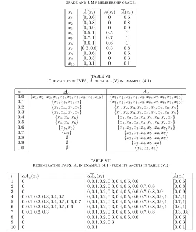
Example 4.1: Let X = {xi|i= 1,2, ...,10}, and Aˆ ∈ ˆ

F(X) is an IVFS defined in Table V. Table VI shows the

α-cuts of IVFSAˆcalculated from its LMF and UMF. Table VII shows how to reconstruct IVFSAˆ knowing itsα-cuts.

Also using equation (20), if Aˆ is a continuous and convex

IVFS i.e. A and A are continuous and convex as seen in

Figure (2). Its α-cut is Aˆα = Aα, Aα

where Aα =

_L

xα,Rxα

andAα=

_L

xα,Rxα

. Then,Aˆα, is calculated using the following formula:

ˆ

Aα=

_L

xα,Rxα

,_L

xα,Rxα

, α≤h(A)

∅,L_x

TABLE V

IVFS,Aˆ_,IN EXAMPLE(4.1). EACH DOMAIN VALUE,x_i,ALONG WITH ITS CORRESPONDING INTERVAL MEMBERSHIP GRADE, LMFMEMBERSHIP GRADE ANDUMFMEMBERSHIP GRADE.

xi Aˆ(xi) A(xi) A(xi)

x1 [0,0.6] 0 0.6

x2 [0,0.8] 0 0.8

x3 [0,0.9] 0 0.9

x4 [0.5,1] 0.5 1

x5 [0.7,1] 0.7 1

x6 [0.6,1] 0.6 1

x7 [0.3,0.8] 0.3 0.8

x8 [0,0.6] 0 0.6

x9 [0,0.3] 0 0.3

x10 [0,0.1] 0 0.1

TABLE VI

THEα-CUTS OFIVFS,Aˆ,OF TABLE(V)IN EXAMPLE(4.1).

α Aα Aα

0.0 {x1, x2, x3, x4, x5, x6, x7, x8, x9, x10} {x1, x2, x3, x4, x5, x6, x7, x8, x9, x10}

0.1 {x4, x5, x6, x7} {x1, x2, x3, x4, x5, x6, x7, x8, x9, x10}

0.2 {x4, x5, x6, x7} {x1, x2, x3, x4, x5, x6, x7, x8, x9}

0.3 {x4, x5, x6, x7} {x1, x2, x3, x4, x5, x6, x7, x8, x9}

0.4 {x4, x5, x6} {x1, x2, x3, x4, x5, x6, x7, x8}

0.5 {x4, x5, x6} {x1, x2, x3, x4, x5, x6, x7, x8}

0.6 {x5, x6} {x1, x2, x3, x4, x5, x6, x7, x8}

0.7 {x5} {x2, x3, x4, x5, x6, x7}

0.8 ∅ {x2, x3, x4, x5, x6, x7}

0.9 ∅ {x3, x4, x5, x6}

1.0 ∅ {x4, x5, x6}

TABLE VII

REGENERATINGIVFS,Aˆ,IN EXAMPLE(4.1)FROM ITSα-CUTS IN TABLE(VI)

i αA_α(xi) αAα(xi) Aˆ(xi)

1 0 0,0.1,0.2,0.3,0.4,0.5,0.6 [0,0.6] 2 0 0,0.1,0.2,0.3,0.4,0.5,0.6,0.7,0.8 [0,0.8] 3 0 0,0.1,0.2,0.3,0.4,0.5,0.6,0.7,0.8,0.9 [0,0.9] 4 0,0.1,0.2,0.3,0.4,0.5 0,0.1,0.2,0.3,0.4,0.5,0.6,0.7,0.8,0.9,1 [0.5,1] 5 0,0.1,0.2,0.3,0.4,0.5,0.6,0.7 0,0.1,0.2,0.3,0.4,0.5,0.6,0.7,0.8,0.9,1 [0.7,1] 6 0,0.1,0.2,0.3,0.4,0.5,0.6 0,0.1,0.2,0.3,0.4,0.5,0.6,0.7,0.8,0.9,1 [0.6,1] 7 0,0.1,0.2,0.3 0,0.1,0.2,0.3,0.4,0.5,0.6,0.7,0.8 [0.3,0.8] 8 0 0,0.1,0.2,0.3,0.4,0.5,0.6 [0,0.6]

9 0 0,0.1,0.2,0.3 [0,0.3]

10 0 0,0.1 [0,0.1]

where∀α:Lxα≤Lxα≤Rxα≤Rxα,h(A) = sup∀xA(x) is the height of LMF, and ∅ is an Empty Set. Another way of defining α-cuts for IVFSs is the method provided by Kaufmann and Gupta [15]. For example consider the same set provided in equation (22), theα-cuts are described in the following way, i.e.,

ˆ

AKGα =

_L

xα,Lxα

,_R

xα,Rxα

, α < h(A) _L

xα,Rxα

, α≥h(A) (23)

There are two drawbacks to this method. Firstly, it does not reduce to the α-cut of FSs directly, instead some ma-nipulation and rearrangement must be done and secondly, it does not hold the semantics of α-cuts through out the representation. In equation (23), what does x∈_L

xα,Lxα

represent? It has a rather complicated relationship to LMF and UMF. It is the values xof the domain that belongs to Aα and does not belong to non boundary elements of Aα, i.e.,

ˆ

Aα=

x|x∈Aα andx /∈

Aα−

inf

∀xAα,sup∀x

Aα

=

x∈L_x α,Rxα

andx /∈ L_x α,Rxα

=Aα∩A

′

α+

(24)

where the minus sign − represents the set difference,

L_x α,Rxα

is an open interval, andA′α+ is the complement of the strong α-cut (α+_{) of the LMF A. Zeng et al. [36],}

particular case, i.e.,

ˆ

Aα=x|A(x)≥α, A(x)≥α (25)

Equation 25 is a generalisation of the α-cuts for FSs. There is no distinction between the domain values that belong to the α-cuts of the LMF and the UMF. Hence, theα-cut is a crisp set rather than a pair. Yager [32] also defined a closely related definition for the discrete cases, which can easily be generalised for continuous cases. Although there are different ways to define α-cuts for IVFSs, the representation theorem is the same. The ability to extend operations using theα-cut RT is what makes it useful.

Theorem 4.2 (IVFS α-EP): Let, X =X1×...×Xn, be the Cartesian product of universes, andAˆ1, ...,Aˆn be IVFSs in each universe respectively. Also letY be another universe andBˆ ∈Y be an IVFS such thatBˆ =f( ˆA1, ...,Aˆn), where

f :X→Y is a monotonic mapping. Then,Bˆ, is equal to the union of applying the same function to all the decomposed α-cuts of the IVFSs [12], i.e.,

ˆ

B=f( ˆA1, ...,Aˆn)

=[

∀α

α f(A_1α, ..., A_nα), f(A1α, ..., Anα)

(26)

Proof. SinceA1, ..., An, A1, ..., An∈F(X), then from equa-tion (2)

f(A1, ..., An) = [

∀α

αf(A1α, ..., Anα)

f(A1, ..., An) =

[

∀α

αf(A1α, ..., Anα)

Therefore, we have

f( ˆA1, ...,Aˆn) = f(A1, ..., An), f(A1, ..., An)

= [

∀α

αf(A_1α, ..., A_nα),[ ∀α

αf(A1α, ..., Anα) !

=[

∀α

α f(A1α, ..., Anα), f(A1α, ..., Anα)

which completes the proof. The following example shows

how to perform the union and intersection of IVFSs using α-cuts.

Example 4.2: Let ˆ4 andˆ8 be two IVFS defined in Table VIII and Table IX, respectively. The α-cuts of both their

LMF and UMF is shown in Table X. The union of the α

-cuts are shown in Table XI. This will eventually lead to an IVFS ˆ4∪ˆ8. The method used to generate the membership grades of ˆ4∪ˆ8 from itsα-cuts is shown in Table XII. The intersection of theα-cuts are shown in Table XIII. This will eventually lead to an IVFSˆ4∩ˆ8. The method used to generate the membership grades ofˆ4∩ˆ8from its α-cuts is shown in Table XIV.

To summarise the overall picture, we view the process of deriving operations for IVFSs to involve the definition of these operations for two distinct FSs, i.e., the UMF and LMF. The same operations can be defined for crisp sets (or intervals) and then extend them to FSs using theα-EP. The obvious conclusion is to define these operations for IVFSs by taking both FSs and using theα-EP. To derive operations for IVFSs in such a simple and elegant process is in itself, we believe, a significant result.

V. ALPHA-CUTS OFTYPE-2 FUZZYSETS

A. α-cut Representation Theorem

In the previous section we discussed α-cuts for IVFSs. These α-cuts can be defined in different ways. What is important, is that these are crisp sets and the IVFS α -EP extends operations directly from crisp sets to IVFSs. This fact is crucial since in Section III we showed that α -planes are IVFSs, and developed the α-PEP to allow us to extend operations from IVFSs to T2FSs. Combining these two theorems lead us to define α-cuts for T2FSs, directly. First, we define the UMF and LMF of α-planes.

Definition 5.1: Let, A˜ ∈ F˜(X), be a T2FS and, A˜α˜ ∈

ˆ

F(X), be a IVFS representing its α-plane at level α˜, such thatA˜α˜=ux,α˜, ux,α˜. Let,Aα˜ ∈F(X), be the LMF ofA˜α˜

and ,Aα˜ ∈F(X), be the UMF ofA˜α˜. Then eachα-plane is

completely determined by its LMF and UMF, i.e.,

˜

Aα˜= Aα˜, Aα˜

(27)

where A˜α(˜ x) = Aα˜(x), Aα(˜ x), Aα˜(x) = ux,α˜ and

Aα(˜ x) =ux,α˜.

It is clear that both the LMF and UMF are FSs. Now, let us take the α-cuts of each α-plane.

Definition 5.2 (T2α-cuts): Let,A˜∈F˜(X), be a T2FS and, ˜

Aα˜= Aα˜, Aα˜, be itsα-plane at levelα˜ represented by its

LMF and UMF. Then, A˜α,α˜ , is the α-cut of thatα-plane at

level α, i.e.,

˜

Aα,α˜ = Aα,α˜ , Aα,α˜

(28)

where Aα,α˜ andAα,α˜ are theα-cuts of the LMF and UMF

of α-plane,A˜α˜, respectively.

The LMF and UMFα-cuts are crisp sets since the LMF and UMF are FSs. Hence, Aα,α˜ (x) ∈ {0,1}, and Aα,α(˜ x) ∈ {0,1}. Following definition (4.2) we defineα-IVFS of each α-cut, i.e.,

Definition 5.3: For each α-cut, A˜α,α˜ , of the T2FS,A˜, a

special IVFS (α-IVFS), αA˜α,α˜ ∈ Fˆ(X), can be defined as

follows:

αA˜α,α˜ =α Aα,α˜ , Aα,α˜

= αAα,α˜ , αAα,α˜

TABLE VIII IVFS,ˆ4,INEXAMPLE4.2.

x 2 3 4 5 6

ˆ

4(x) [0,0.2] [0.4,0.6] [0.8,1] [0.5,0.6] [0,0.4]

TABLE IX IVFS,ˆ8,INEXAMPLE4.2.

x 5 6 7 8 9 10 11

ˆ

8(x) [0,0.1] [0.2,0.5] [0.6,0.8] [1,1] [0.5,0.8] [0.2,0.4] [0,0.1]

TABLE X

THEα_-CUTS OFIVFS,ˆ4ANDˆ8,INEXAMPLE4.2.

α 4_α 8_α 4α 8α

0.0 {2,3,4,5,6} {5,6,7,8,9,10,11} {2,3,4,5,6} {5,6,7,8,9,10,11} 0.1 {3,4,5} {6,7,8,9,10} {2,3,4,5,6} {5,6,7,8,9,10,11} 0.2 {3,4,5} {6,7,8,9,10} {2,3,4,5,6} {6,7,8,9,10} 0.3 {3,4,5} {7,8,9} {3,4,5,6} {6,7,8,9,10} 0.4 {3,4,5} {7,8,9} {3,4,5,6} {6,7,8,9,10} 0.5 {4,5} {7,8,9} {3,4,5} {6,7,8,9} 0.6 {4} {7,8} {3,4,5} {7,8,9}

0.7 {4} {8} {4} {7,8,9}

0.8 {4} {8} {4} {7,8,9}

0.9 ∅ {8} {4} {8}

1.0 ∅ {8} {4} {8}

TABLE XI

THEα_-CUTS OFIVFS,ˆ4∪ˆ_8,INEXAMPLE4.2.

α 4_α∪8_α 4α∪8α

0.0 {2,3,4,5,6,7,8,9,10,11} {2,3,4,5,6,7,8,9,10,11} 0.1 {3,4,5,6,7,8,9,10} {2,3,4,5,6,7,8,9,10,11} 0.2 {3,4,5,6,7,8,9,10} {2,3,4,5,6,7,8,9,10} 0.3 {3,4,5,7,8,9} {3,4,5,6,7,8,9,10} 0.4 {3,4,5,7,8,9} {3,4,5,6,7,8,9,10} 0.5 {4,5,7,8,9} {3,4,5,6,7,8,9} 0.6 {4,7,8} {3,4,5,7,8,9} 0.7 {4,8} {4,7,8,9} 0.8 {4,8} {4,7,8,9}

0.9 {8} {4,8}

1.0 {8} {4,8}

where αA˜α,α(˜ x) =α∧

Aα,α˜ (x), Aα,α(˜ x)

.

It is noticeable that αAα,α˜ and αAα,α˜ are special FSs (α

-FS). The union of allα-IVFSs constitute anα-plane.

˜

Aα˜=

[

∀α

αA˜α,α˜

=[

∀α

α Aα,α˜ , Aα,α˜

(30)

Earlier in Equation 13 we defined a special T2FS (α-T2FS) associated with each α-plane, α˜A˜α˜. We make use of this

definition again.

˜

αA˜α˜= ˜α

[

∀α

αA˜α,α˜

= ˜α[ ∀α

α Aα,α˜ , Aα,α˜

(31)

where α˜S

∀ααA˜α,α(˜ x)

(ux,α)˜ = α˜ ∧

S

∀ααA˜α,α(˜ x)

(ux,α)˜ and S∀ααA˜α,α(˜ x)(ux,α) = 1˜ if

ux,α˜ ∈ S∀ααA˜α,α(˜ x) and zero otherwise. It is already known from theα-plane representation theorem that a T2FS can be represented by the union of all suchα-T2FSs.

Theorem 5.1 (T2FSα-cut RT): A T2FS,A˜, can be repre-sented by the union of all its α-T2FSs, i.e.,

˜

A=[

∀α˜

˜

α[

∀α

αA˜α,α˜ (32)

Proof. Straight forward substitute equation (31) in equation

(14) of theorem (4.1). The α-cut representation allow

-TABLE XII

IVFS,ˆ4∪ˆ_8,INEXAMPLE4.2FROM ITSα_-CUTS INTABLEXI.

x α(4∪8)α(x) α(4∪8)α(x) ˆ4∪ˆ8

(x)

2 0 0,0.1,0.2 [0,0.2]

3 0,0.1,0.2,0.3,0.4 0,0.1,0.2,0.3,0.4,0.5,0.6 [0.4,0.6] 4 0,0.1,0.2,0.3,0.4,0.5,0.6,0.7,0.8 0,0.1,0.2,0.3,0.4,0.5,0.6,0.7,0.8,0.9,1 [0.8,1] 5 0,0.1,0.2,0.3,0.4,0.5 0,0.1,0.2,0.3,0.4,0.5,0.6 [0.5,0.6] 6 0,0.1,0.2 0,0.1,0.2,0.3,0.4,0.5 [0.2,0.5] 7 0,0.1,0.2,0.3,0.4,0.5,0.6 0,0.1,0.2,0.3,0.4,0.5,0.6,0.7,0.8 [0.6,0.8] 8 0,0.1,0.2,0.3,0.4,0.5,0.6,0.7,0.8,0.9,1 0,0.1,0.2,0.3,0.4,0.5,0.6,0.7,0.8,0.9,1 [1,1] 9 0,0.1,0.2,0.3,0.4,0.5 0,0.1,0.2,0.3,0.4,0.5,0.6,0.7,0.8 [0.5,0.8] 10 0,0.1,0.2 0,0.1,0.2,0.3,0.4 [0.2,0.4]

11 0 0,0.1 [0,0.1]

TABLE XIII

THEα_-CUTS OFIVFS,ˆ4∩ˆ_8,INEXAMPLE4.2. α 4_α∩8_α 4α∩8α

0.0 {5,6} {5,6} 0.1 ∅ {5,6}

0.2 ∅ {6}

0.3 ∅ {6}

0.4 ∅ {6}

0.5 ∅ ∅

0.6 ∅ ∅

0.7 ∅ ∅

0.8 ∅ ∅

0.9 ∅ ∅

1.0 ∅ ∅

TABLE XIV

IVFS,ˆ4∩ˆ_{8,INEXAMPLE4.2FROM ITS}α-CUTS INTABLEXIII

x α(4∩8)α(x) α(4∩8)α(x) ˆ4∩ˆ8

(x)

5 0 0,0.1 [0,0.1]

6 0 0,0.1,0.2,0.3,0.4 [0,0.4]

cut representations are by definition related. The relationship between these representations is depicted in Figure 4. The

˜ A

S ∀x

x,A˜x

˜ A

x

=

S

∀ ˜ α

˜ α_A˜

x_, ˜

α S

∀˜αα˜A˜˜α ˜

Aα˜= S ∀α

αA˜˜α, α S

∀α˜α˜ S

∀ααA˜˜α,α Verti

cal S lice

α

-p

la

n

e

α_-cu

t Cris_{p se}

ts

Fuzz yse

ts

IV

F

S

s

Fig. 4. The vertical slice,α_{-plane and}α_{-cut representations of T2FSs and} their relationship.

relation between domain values in the classical set theoretic way is behind the idea of α-cuts for FSs. This relation is maintained across IVFSs and T2FSs as they are extension of classical FSs. What makes such decomposition interesting is the ability to perform operations in the classical set theoretic sense. This is made possible by extending the α-EP of FSs

to IVFSs, and by the α-PEP of α-planes.

Theorem 5.2 (T2FSα-cut EP): Let,X =X1×...×Xn, be the Cartesian product of universes, andA˜1, ...,A˜n be T2FSs in each universe respectively. Also letY be another universe andB˜ ∈Y be a T2FS such thatB˜ =f( ˜A1, ...,A˜n), where

f :X→Y is a monotone mapping. Then B˜ is equal to the union of applying the same function to all its decomposed α-cuts, i.e.,

˜

B=f( ˜A1, ...,A˜n)

=[

∀α˜

˜

α[

∀α

αf( ˜A1α,α˜ , ...,A˜nα,α˜ )

Proof. From theorem (3.2) operations are extended to T2FSs

by the α-PEP from operations on its α-planes which are IVFSs. For eachα-plane theorem (4.2) allows the operations to be extended from crisp sets. Hence, straight forward substitute equation (26) in equation (15) and that completes

the proof. This theorem first appeared in [10]. The

following example demonstrates how to use Theorem 5.2 for defining operations for T2FSs by calculating the join and meet of a T2FS using the α-cut extension principle.

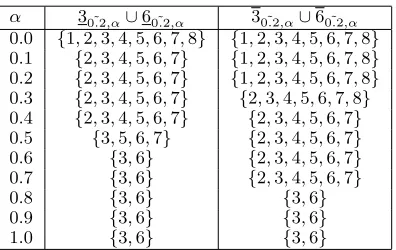
Example 5.1: Consider the T2FSs, ˜3, in Table XV and, ˜

each T2FS into its α-planes and each α-plane to its α-cuts must be performed. Then, for example the union ofα-planes ˜3₀˜_.2∪˜6₀˜_.2, is computed. The interval membership grades of

each α-plane are constructed using the bounds of the PMs Jx,α˜, i.e. Table XVII and Table XVIII. The steps to perform

the union is shown in Table XIX, Table XX and Table XXI. These are the same steps used to perform the union of IVFSs. To perform the union of the T2FSs the same task is repeated for all the α-planes.

In this section we definedα-cuts for T2FSs and its associated T2FSα-EP which allows us to extend operations to FSs and its extensions.

VI. CONCLUSION

In this paper we defined theα-cut decomposition theorem for T2FSs, through the use of the basic ideas ofα-cuts in FSs and the EP. We also showed that this novel decomposition theorem can extend mathematical concepts from crisp sets to T2FSs, directly. In this paper also we investigated a generalisation that allow us to extend operations from IVFSs to T2FSs, through the α-plane RT. In order to clarify these concepts we used several worked examples. It is the authors belief that the novel theories provided in this paper will stim-ulate more investigation and applications of T2FSs. Future work includes taking advantage of the independent nature of theseα-cuts to perform operations on parallel processors, such as graphical processing units (GPUs).

REFERENCES

[1] B. Araabi, N. Kehtarnavaz, and C. Lucas. Restrictions imposed by the fuzzy extension of relations and functions. Journal of Intelligent and Fuzzy Systems, 11(1):9–22, 2001.

[2] H. Bustince, E. Barrenechea, M. Pagola, and J. Fernandez. Interval-valued fuzzy sets constructed from matrices: Application to edge detection. Fuzzy Sets and Systems, 160(13):1819–1840, 2009. [3] O. Castillo and P. Melin. Type-2 Fuzzy Logic: Theory and

Applica-tions, volume 223. Springer-Verlag, Heidelberg, Germany, 1st edition, January 2008. Book (ISBN: 978-3-540-76283-6).

[4] Q. Chen and S. Kawase. On fuzzy-valued fuzzy reasoning. Fuzzy Sets and Systems, 113:237–251, 2000.

[5] S. Coupland and R. John. Geometric type-1 and type-2 fuzzy logic systems. IEEE Transactions on Fuzzy Systems, 15(1):3–15, 2007. [6] J. C. Figueroa Garcia. An approximation method for type reduction

of an interval type-2 fuzzy set based onα_{-cuts. In Computer Science}

and Information Systems (FedCSIS), 2012 Federated Conference on, pages 49–54. IEEE, 2012.

[7] J. C. Figueroa Garcia and G. Hernandez. Solving linear program-ming problems with interval type-2 fuzzy constraints using interval optimization. In IFSA World Congress and NAFIPS Annual Meeting (IFSA/NAFIPS), 2013 Joint, pages 623–628. IEEE, 2013.

[8] S. Greenfield, F. Chiclana, S. Coupland, and R. John. The collapsing method of defuzzification for discretised interval type-2 fuzzy sets. Information Sciences, 179(13):2055–2069, 2009.

[9] H. Hamrawi and S. Coupland. Non-specificity measures for type-2 fuzzy sets. In Proc. FUZZ-IEEE, pages 73type-2–737, Korea, August 2009.

[10] H. Hamrawi and S. Coupland. Type-2 fuzzy arithmetic using alpha-planes. In Proc. IFSA/EUSFLAT, pages 606–611, Portugal, 2009. [11] H. Hamrawi, S. Coupland, and R. John. Extending operations on

type-2 fuzzy sets. In Proc. UKCI, Nottingham, UK, September 2009. [12] H. Hamrawi, S. Coupland, and R. John. A novel alpha-cut representa-tion for type-2 fuzzy sets. In Proc. FUZZ-IEEE, pages 1–8, Barcelona, Spain, July 2010.

[13] R. John. Type-2 fuzzy sets: an appraisal of theory and applications. International Journal of Uncertainty, Fuzziness and Knowledge-Based Systems, 6:563–576, 1998.

[14] R. John and S. Coupland. Type-2 fuzzy logic: A historical view. IEEE Computational Intelligence Magazine, 2(1):57–62, February 2007. [15] A. Kaufmann and M. Gupta. Introduction to Fuzzy Arithmetic Theory

and Applications. Van Nostran Reinhold Co. Inc., 1985.

[16] G. Klir and B. Yuan. Fuzzy Sets and Fuzzy Logic: Theory and Applications. Prentice Hall, Upper Saddle River, NJ, 1995. [17] F. Liu. An efficient centroid type-reduction strategy for general type-2

fuzzy logic system. Information Sciences, 178(9):2224–2236, 2008. [18] J. Mendel. Uncertain Rule-Based Fuzzy Logic Systems: Introduction

and New Directions. Prentice Hall, Upper Saddle River, NJ, 2001. [19] J. Mendel, F. Liu, and D. Zhai.α-plane representation for type-2 fuzzy

sets: Theory and applications. IEEE Transactions on Fuzzy Systems, 17(5):1189–1207, 2009.

[20] J. Mendel and H. Wu. Type-2 fuzzistics for nonsymmetric interval type-2 fuzzy sets: Forward problems. IEEE Transactions on Fuzzy Systems, 15(5):916–930, 2007.

[21] J. M. Mendel. Advances in type-2 fuzzy sets and systems. Information Sciences, 177(1):84–110, January 2007.

[22] J. M. Mendel and R. John. Type-2 fuzzy sets made simple. IEEE Transaction on Fuzzy Systems, 10(2):117–127, 2002.

[23] H. Nguyen. A note on the extension principle for fuzzy sets. J. Mathematical Analysis and Applications, 64(2):369–380, 1978. [24] J. T. Rickard, J. Aisbett, and G. Gibbon. Fuzzy subsethood for fuzzy

sets of type-2 and generalized type-n. IEEE Transactions on Fuzzy Systems, 17(1):50–60, 2009.

[25] J. Starczewski. Efficient triangular type-2 fuzzy logic systems. Inter-national Journal of Approximate Reasoning, 50(5):799–811, 2009. [26] H. Tahayori, A. Tettamanzi, and G. Antoni. Approximated type-2

fuzzy set operations. In Proc. FUZZ-IEEE 2006, pages 9042 – 9049, Vancouver, Canada, July 2006.

[27] C. Wagner and H. Hagras. zSlices–Towards bridging the gap between Interval and General Type-2 Fuzzy Logic. In FUZZ-IEEE 2008., pages 489–497, Hong Kong, 2008.

[28] C. Wagner and H. Hagras. Toward general type-2 fuzzy logic systems based on zslices. IEEE Transactions on Fuzzy Systems, 18(4):637 –660, 2010.

[29] C. Walker and E. Walker. Sets with type-2 operations. International Journal of Approximate Reasoning, 50(1):63–71, 2009.

[30] D. Wu and J. Mendel. Corrections to Aggregation Using the Linguistic Weighted Average and Interval Type-2 Fuzzy Sets. IEEE Transactions on Fuzzy Systems, 16(6):1664–1666, 2008.

[31] D. Wu and J. M. Mendel. Aggregation Using the Linguistic Weighted Average and Interval Type-2 Fuzzy Sets. IEEE Transactions on Fuzzy Systems, 15(6):1145, 2007.

[32] R. R. Yager. Level sets and the extension principle for interval valued fuzzy sets and its application to uncertainy measures. Information Sciences, 178:3565–3576, 2008.

[33] L. A. Zadeh. The concept of a linguistic variable and its application to approximate reasoning-1. Information Sciences, 8:199 – 249, 1975. [34] L. A. Zadeh. The concept of a linguistic variable and its application to approximate reasoning-2. Information Sciences, 8:301 – 357, 1975. [35] L. A. Zadeh. The concept of a linguistic variable and its application to approximate reasoning-3. Information Sciences, 9:43 – 80, 1975. [36] W. Zeng and H. Li. Representation theorem of interval-valued fuzzy

set. International Journal of Uncertainty, Fuzziness and Knowledge-Based Systems, 14(3):259–269, 2006.

TABLE XV

T2FS˜3,INEXAMPLE5.1. THE NUMBERS IN BETWEEN ARE THESGS,˜3x(ux).

x/ux 0.0 0.1 0.2 0.3 0.4 0.5 0.6 0.7 0.8 0.9 1.0

1 1.0 0.6 0.3

2 0.1 0.6 1.0 0.7 0.2

3 1.0

4 0.1 0.6 1.0 0.7 0.2

5 1.0 0.6 0.3

TABLE XVI

T2FS˜6,INEXAMPLE5.1. THE NUMBERS IN BETWEEN ARE THESGS,˜6x(ux).

x/ux 0.0 0.1 0.2 0.3 0.4 0.5 0.6 0.7 0.8 0.9 1.0

4 1.0 0.8 0.4 0.2 0.1

5 0.2 1.0 0.4

6 1.0

7 0.2 1.0 0.4

8 1.0 0.8 0.4 0.2 0.1

TABLE XVII

α-PLANE,ˆ30˜.2,INEXAMPLE5.1.

x 1 2 3 4 5

˜

30˜.2(x) [0,0.2] [0.4,0.7] [1,1] [0.4,0.7] [0,0.2]

TABLE XVIII α-PLANE,˜60˜.2,INEXAMPLE5.1.

x 4 5 6 7 8

˜

60˜.2(x) [0,0.3] [0.5,0.7] [1,1] [0.5,0.7] [0,0.3]

Hussam Hamrawi Hussam Hamrawi has been Assistant Professor of Computer and Systems En-gineering at AAUT, Merowe, Sudan since May 2015. Prior to this he held the post of Assistant Professor of Intelligent Systems at the University of Bahri, Sudan from September 2011. His area of expertise is fuzzy logic, obtaining his PhD in this subject from De Montfort University in 2011.

Simon Coupland Simon Coupland has worked at the Centre for Computational Intelligence at De Montfort University, UK since 2005, completing his PhD there in 2006. His area of expertise is type-2 fuzzy logic and application of computa-tional intelligence approach more generally. He has chaired many conference session on type-2 fuzzy logic and reviews paper for a number of international journals in this field.

TABLE XIX

THEα_-CUTS OFα_-PLANES,˜30˜.2AND˜60˜.2,INEXAMPLE5.1.

α 30˜.2,α 60˜.2,α 30˜.2,α 60˜.2,α

0.0 {1,2,3,4,5} {4,5,6,7,8} {1,2,3,4,5} {4,5,6,7,8} 0.1 {2,3,4} {5,6,7} {1,2,3,4,5} {4,5,6,7,8} 0.2 {2,3,4} {5,6,7} {1,2,3,4,5} {4,5,6,7,8} 0.3 {2,3,4} {5,6,7} {2,3,4} {4,5,6,7,8} 0.4 {2,3,4} {5,6,7} {2,3,4} {5,6,7} 0.5 {3} {5,6,7} {2,3,4} {5,6,7} 0.6 {3} {6} {2,3,4} {5,6,7} 0.7 {3} {6} {2,3,4} {5,6,7}

0.8 {3} {6} {3} {6}

0.9 {3} {6} {3} {6}

1.0 {3} {6} {3} {6}

TABLE XX

THEα-CUTS OFα-PLANES,˜30˜.2∪˜60˜.2,INEXAMPLE5.1.

α 30˜_.2_,α∪60˜_.2_,α 30˜.2,α∪60˜.2,α

0.0 {1,2,3,4,5,6,7,8} {1,2,3,4,5,6,7,8} 0.1 {2,3,4,5,6,7} {1,2,3,4,5,6,7,8} 0.2 {2,3,4,5,6,7} {1,2,3,4,5,6,7,8} 0.3 {2,3,4,5,6,7} {2,3,4,5,6,7,8} 0.4 {2,3,4,5,6,7} {2,3,4,5,6,7} 0.5 {3,5,6,7} {2,3,4,5,6,7} 0.6 {3,6} {2,3,4,5,6,7} 0.7 {3,6} {2,3,4,5,6,7}

0.8 {3,6} {3,6}

0.9 {3,6} {3,6}

1.0 {3,6} {3,6}

TABLE XXI

α_-PLANE,˜30˜.2,α∪˜60˜.2,α,INEXAMPLE5.1FROM ITSα-CUTS INTABLEXX.

x α(30˜.2,α∪60˜.2,α)(x) α(30˜.2,α∪60˜.2,α)(x) ˜30˜.2,α∪˜60˜.2,α

(x)

1 0 0,0.1,0.2 [0,0.2]

2 0,0.1,0.2,0.3,0.4 0,0.1,0.2,0.3,0.4,0.5,0.6,0.7 [0.4,0.7] 3 0,0.1,0.2,0.3,0.4,0.5,0.6,0.7,0.8,0.9,1 0,0.1,0.2,0.3,0.4,0.5,0.6,0.7,0.8,0.9,1 [1,1] 4 0,0.1,0.2,0.3,0.4 0,0.1,0.2,0.3,0.4,0.5,0.6,0.7 [0.4,0.7] 5 0,0.1,0.2,0.3,0.4,0.5 0,0.1,0.2,0.3,0.4,0.5,0.6,0.7 [0.5,0.7] 6 0,0.1,0.2,0.3,0.4,0.5,0.6,0.7,0.8,0.9,1 0,0.1,0.2,0.3,0.4,0.5,0.6,0.7,0.8,0.9,1 [1,1] 7 0,0.1,0.2,0.3,0.4,0.5 0,0.1,0.2,0.3,0.4,0.5,0.6,0.7 [0.5,0.7]