Formability optimisation of fabric preforms by controlling material draw in through in plane constraints

Formability optimisation of fabric preforms by controlling

material draw-in through in-plane constraints

S Chen, L T Harper*_{, A Endruweit, N A Warrior}

Polymer Composites Group, Division of Materials, Mechanics and Structures, Faculty of Engineering, University of Nottingham, UK, NG7 2RD

*_{[email protected] , Tel +44 (0)115 9513823}

Abstract

A genetic algorithm is coupled with a finite element model to optimise the arrangement

of constraints for a composite press-forming study. A series of springs are used to locally

apply in-plane tension through clamps to the fibre preform to control material draw-in.

The optimisation procedure seeks to minimise local in-plane shear angles by determining

the optimum location and size of constraining clamps, and the stiffness of connected

springs. Results are presented for a double-dome geometry, which are validated against

data from the literature. Controlling material draw-in using in-plane constraints around

the blank perimeter is an effective way of homogenising the global shear angle

distribution and minimising the maximum value. The peak shear angle in the

double-dome example was successfully reduced from 48.2 to 37.2 following a two-stage

optimisation process.

Keywords

1 Introduction

In the manufacture of composite components, draping of reinforcement fabrics can cause

large local shear deformations (change in fibre orientations, fibre volume fraction, fabric

thickness, etc.) to occur. For most fabrics, in-plane shear is the main deformation

mechanism in drape, but excessive local shear can lead to wrinkling (i.e. out-of-plane

buckling due to local compressive stresses) and fibre fracture [1]. To successfully drape

a reinforcement without encountering unwanted wrinkles and defects, the main challenge

is identifying optimum forming conditions. Among the processing parameters affecting

fabric press forming, the distribution of the blank holder force (BHF) and the blank shape

are two essential properties that should be optimised to improve the quality of the formed

shape [2, 3]. To optimise these parameters, efforts have been made to develop simulation

tools to facilitate parametric studies.

Kinematic drape simulation codes [4, 5] use a purely geometrical approach to compute

fabric drape patterns, but whilst this method is computationally relatively inexpensive,

there is no accounting for mechanical material properties or process conditions.

Conversely, Finite Element (FE) simulations enable the physics of the forming problem

to be modelled and are becoming a viable choice as computing resources improve. This

approach enables the influence of process parameters, including contacts and friction

between components to be studied, but more importantly can be used to indicate the

likelihood of defects occurring during forming. To date, most FE forming studies have

focused on capturing the deformation of fabrics accurately though implementation of

suitable constitutive material models [6, 7], rather than focusing on optimising the

Procedures for optimisation of the forming process can be classified as direct or indirect.

Indirect methods refer to trial and error approaches, which require experience to interpret

the results and can be time consuming. Nonetheless, they are likely to be used for

optimising composite forming processes, since the complex relationship between

wrinkling strain and clamping force does not need to be formulated. Indirect methods

have previously been used to optimise fabric blank size [2] and BHF distribution [3], in

order to minimise wrinkle formation. The probability for wrinkles to occur was shown to

increase as the blank size is reduced relative to the size of the punch, since the tension in

the blank is released during the latter stage of the forming process [2]. A uniform BHF

distribution produced the least wrinkles in forming a hemisphere. However, it was

concluded that a segmented blank holder is required to further reduce the level of

wrinkling, to vary the local pressure distribution as a function of intra-ply shear and

compressive forces [3].

Direct optimisation methods rely on mathematical relationships between the processing

parameters (BHF, blank shape, fabric pre-shear) and the objective function (describing

shear angle, wrinkling etc.) to be formulated, and have been used extensively for

optimising metal forming problems. They commonly employ Genetic Algorithms (GA)

[8-11], which mimic natural selection processes to enable the strongest permutation of

design variables to evolve, and inferior ones to fade out. GAs are not widely used for

optimising composite forming problems, because they are computationally expensive. A

GA was coupled with a kinematic drape model by Skordos et al. [5], where the drape start

point, drape direction and the pre-shear angle of the fabric were defined as design

parameters. Employing the GA reduced the CPU time to 30 % of that required for an

a GA to optimise the BHF around the perimeter of the blank, with the objective of

minimising wrinkling [12]. Results indicated that optimising the BHF successfully

eliminated concentrated buckling of tows around the base of the hemisphere, without

affecting the in-plane shear angle distribution.

This paper presents a GA coupled with a non-linear explicit FE model to optimise the

draw-in of the blank during composite press-forming. Spring-loaded clamps are used to

directly provide in-plane tension to the fabric, rather than applying a normal pressure

(resulting in in-plane friction) through a blank holder. This technique has been discussed

in the literature for thermoplastic forming [13, 14] and is currently used in the automotive

industry in preforming of non-crimp fabric. It enables the blank to be heated easily if the

fabric is bindered or pre-impregnated, as the clamps are situated outside of the heated

region of the press. This arrangement also offers more flexibility in terms of controlling

material draw-in, as the spring-loading for each clamp can be controlled independently,

but results in increased complexity. The optimisation procedure seeks to determine the

optimum location and size of each clamp and the stiffness of each spring controlling the

local draw-in. The objective is to minimise the global in-plane shear angle of the fabric.

2 Modelling of fabric preforming using in-plane constraints

2.1 Fabric material model

A non-orthogonal constitutive model is employed in this work to describe the fabric

behaviour during preforming, which was previously derived by the authors [15]. This

macro-scale model was shown to effectively capture the dominant factors in fabric

forming, including in-plane shear, fibre elongation and inter-tow/intra-ply slipping. This

because it appropriately describes the anisotropic behaviour of biaxial materials under

large shear deformation [17, 18]. A VFABRIC subroutine was developed in

Abaqus/Explicit to implement the mechanical constitutive relations for woven fabrics.

Comparisons against experimental data [15] indicated high levels of accuracy for the

simulation results, which was not significantly compromised by time-scaling or

mass-scaling employed to reduce CPU time.

2.2 Validation for forming model using in-plane constraints

Numerical tests have been performed to validate the material model against experimental

data for the case where in-plane constraints are used to provide tension in the fabric to

control draw-in [13, 18], rather than out-of-plane blank-holders. Material parameters

were consistent with the values in the literature [19-22] for a balanced plain weave glass

fibre/polypropylene commingled fabric. The value of Young’s modulus was taken to be

35.4 GPa in each fibre direction and the shear modulus was described by a polynomial:

MPa 0.1948) + | | 1.5928 -| | 6.3822 + | | 9.8228 -| | (6.7135

= ₁₂ 4 ₁₂ 3 ₁₂ 2 ₁₂

12    

G (1)

where12is the in-plane shear angle in radians.

Validation was conducted using the same geometry and material properties as in the

literature [13, 18]. The blank was a single 0°/90° ply at a thickness of 0.4 mm. The

optimised blank shape described by Harrison et al. [13] was employed, and the ply was

modelled using quadrilateral membrane elements (M3D4R). Tooling was considered to

be rigid; Coulomb friction was adopted for both tooling-material and material-material

contacts, with a coefficient of 0.2; displacement boundary conditions were applied to the

punch, whilst in-plane spring elements were used to connect the edge of the blank to a

elements was 0.20 N/mm on the short edges and 0.27 N/mm on the long edges of the

rectangular frame [13].

A comparison of the shear angle distributions is presented in Fig. 1. Qualitatively, the

outline shape of the final formed part from the simulation is in very close agreement with

experimental data [13]. A quantitative analysis was performed by comparing the local

shear angle at 20 discrete locations (Table 1). Two experimental repeats were performed

[13], and the measurements from each of the four quadrants were averaged for each repeat.

Fig. 1 indicates that the predicted shear angles from the numerical solution fall within the

range of the experimental values, with deviations of generally less than 2according to

Table 1.

3 Methodology of in-plane constraint optimisation

3.1 General strategy

The initial blank size for the double-dome forming study discussed here was 470 mm ×

270 mm with a thickness of 0.4 mm, and the ply was discretised into 5076 square

membrane elements (M3D4R). The initial fibre orientations in the blank were at 0°/90°.

Springs are arranged around the perimeter of the preform to control material draw-in,

providing in-plane constraints during draping. The optimum design of this system is

dependent on the geometrical arrangement (number, position and size) of the springs and

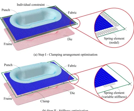
their mechanical properties (stiffness). The optimisation procedure is split into two stages

as shown in Fig. 2: (a) Step I: Clamping arrangement optimisation, (b) Step II: Spring

stiffness optimisation. The first step determines sensible clamping positions to improve

formability, by reducing the maximum global shear angle in the model. Compromises

step determines optimum spring stiffnesses for the derived spring arrangement, therefore

the final solution may not be the global optimum, but near-optimal.

This multi-stage approach makes the procedure independent of specific geometrical

parameters, thus providing the flexibility for application to a variety of test geometries.

Simultaneous optimisation could potentially be more cost-effective computationally and

produce a more efficient solution, but only if a suitable mathematical description could

be derived. However, this would require a specific new formulation of the optimisation

problem for each forming task and would not enable routine application of the method.

3.2 Step I: Clamping arrangement optimisation

Each node around the perimeter of the blank is initially constrained by an individual

spring element with the same initial stiffness (see Fig. 2a). The other end of the spring is

fixed to a fully constrained rigid frame. The force constraining movement of the blank is

always oriented along the spring element axis, extending the spring as the material draws

into the tool while forming. The status of each node (i.e. constrained or unconstrained) is

determined by the optimisation algorithm. When it is unconstrained, the spring element

is removed.

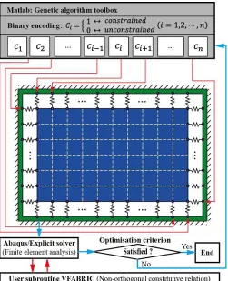
The clamping arrangement optimisation is implemented using Matlab, as shown in Fig.

3. For each loop or “generation” in the GA, a group of constraint patterns called

“individuals” is generated and Abaqus/Explicit input files are produced. The shear angle

distribution in the deformed blank for each individual is determined from Abaqus/Explicit

analyses and then returned to Matlab. The corresponding fitness value is determined from

A binary encoding method is applied to formulate each individual in-plane constraining

pattern for the optimisation algorithm. Each pattern represents a binomial-status series,

which can be described numerically by the encoding scheme in Fig. 3. Each bit in the

binary code represents one potential constraint position and its value corresponds to an

“unconstrained” or “constrained” status (0 or 1). By using this encoding scheme, the

physical problem can be converted into a mathematical problem to perform a series of

GA manipulations to heuristically search for the optimum constraining pattern.

This geometry optimisation problem can be written as:

minimise f{c₁,c₂,...,c_n;₁₂(x,y,z)}

subject to ( 1,2,..., )

ned unconstrai , 0 d constraine , 1 n i

ci 

    (2) ] 90 , 0 [ ) , , (

12 x y z   



M

z y

x, , ) (

wheref{.} is the GA fitness function to describe the selection criterion of the constraining

pattern, which is employed to assess the distribution of shear angles in the material field.

The variableciis theith optimisation variable, which denotes the constrained status at the

ith potential position.݊is the total number of potential positions, i.e. the number of nodes

on the blank perimeter.

The fitness function is used to assess how well each individual constraining pattern has

adapted to the assessment criteria. Its value reflects the relative distance from the

optimum solution, where a smaller value is preferred. A maximum value criterion

(MAXVC) has been adopted here due to faster convergence compared with the Weibull

distribution quantile criterion (WBLQC) previously used [15], whilst maintaining

locking angle, by minimising the maximum shear angle. The maximum can be derived

from the finite element approximation for12(x,y,z). Thus,

} { max } ) , , ( { max )} , , ( ; , ... , , { , ... , 2 , 1 12 ) , , ( 12 2 1 i N i z y x n

MAXVC c c c x y z x y z

f M         (3)

wherefMAXVC{.} denotes the fitness function using MAXVC, which aims to minimise the

maximum shear angle;Mis the spatial material region;12(x,y,z) is the continuous shear

angle distribution in the material region,M;Nis the total number of integration points;

is the absolute value of the variable;i=12(x,y,z)is the absolute value of the shear

angle at theith material point, (xi,yi,zi). Since the constraining pattern influences the shear

angle distribution, the value offMAXVCis used for quantitative assessment of the fitness.

The theoretical optimum positions from Step I cannot be directly used in Step II. It is

impractical to constrain the end of each individual yarn around the perimeter of the blank

in reality, thus neighbouring constraints need to be grouped together to form consolidated

clamps. If the distance between two adjacent constrained positions is smaller than a

threshold value, they are considered to be part of the same clamp. A minimum clamp size

is also specified, and any isolated constraints are discarded. Additionally, clamps are

removed or split if they generate excessive curvature around the perimeter of the blank

or increase MAXVC. The stiffness of each constraint is directly obtained by summing the

stiffnesses of all parallel springs associated with each individual clamp. These

compromises are essential for successful industrial implementation, but their negative

impact can be alleviated to some extent by optimising the spring properties in Step II.

Here, these practical considerations have been implemented manually, which is facilitated

by the two-stage optimisation approach. Whilst it would be feasible to include them in

the optimisation code as additional constraints or regularisation terms, as previously

objective function. This would largely reduce the efficiency in automatically creating FE

models, and the number of geometry variables may change during the optimisation,

significantly increasing complexity. A potential solution would be to define a large

enough number of variables and reserve sufficient memory, but this would be wasteful,

causing computational resources to become redundant.

Since all nodes along the edges were initially connected to springs in Step I, it was

necessary to choose a relatively low starting stiffness from the available range to avoid

over-constraining the blank. In this step, the constraint stiffness was set to 0.03 N/mm at

each applied position.

3.3 Step II: Spring stiffness optimisation

In-plane constraints are applied at the selected clusters of nodes identified in Step I (see

Fig. 2b). A subsequent optimisation step is performed using a GA to determine optimum

stiffness values for each spring from a user-defined range.

For simplification, only linear behaviour is considered, which can be parameterised as

) , ... , 2 , 1

(i m

d k

F ict

ct i ct

i   (4)

where m is the number of constrained clamping positions after refinement, kict is the

stiffness of theith spring,dictis the in-plane displacement at theith constrained position,

andFictis the corresponding constraining force. Consequently, the optimisation variables

are converted into a stiffness kict (i = 1, 2, … , m). This method is also suitable for

modelling non-linear behaviour, as the optimisation method is intrinsically the same, but

the number of parameters increases.

The optimisation problem in Step II can be described as

minimise f{k1 ,k2 ,...,k ; 12(x,y,z)}

ct m ct

subject to k [(k ) ,(kict)upp] (i 1,2,...,m)

low ct i ct

i  

where [(kict)low,(kict)upp] is the applicable stiffness range of the ith constraint. Similarly,

MAXVC is employed again as the fitness function to minimise the maximum shear angle

in Step II

} { max } ) , , ( { max )} , , ( ; , ... , , { , ... , 2 , 1 12 ) , , ( 12 2 1 i N i z y x ct m ct ct

MAXVC k k k x y z x y z

f M         (5)

In this step, optimisation is aimed at finding a near-optimal solution to reduce the negative

influence induced by manually refining the constrained positions. A summary of the GA

is presented in Fig. 4.

3.4 GA stability analysis

The stability of a GA in delivering an optimum solution depends on the diversity of the

population. This is determined by the population size, the initial population and

probabilities for crossover and mutation. The population size has been chosen to be

greater than the number of optimisation variables, for example using 100 for Step I (76

variables corresponding to 76 clamping positions per quarter model). The initial

population is determined randomly to ensure sufficient diversity. The crossover

probability (i.e. the proportion of each population where genes from individuals in the

previous generation are recombined) was 0.8, a compromise between evolution rate and

solution accuracy. The mutation probability enables a small random variation in the

individuals of each generation to create new genes, ensuring genetic diversity and

enhancing the probability for an improved fitness score. Its value was determined

adaptively for this study, based on the fitness scores from the previous generation.

It is important to ensure that the initial population is distributed across the entire solution

individuals in the solution space is therefore measured to quantify the diversity of the

population. For the example of the 76 variables in Step I, the average distance between

individuals must be less than the maximum value of 8.7 (i.e. 761/2_{for 76 binary variables).}

Furthermore, the average distance should progressively decrease for subsequent

generations, indicating a reduction in search space and convergence towards the global

optimum.

4 Results and discussion

4.1 Clamping arrangement optimisation from Step I

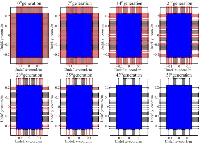
Several generations of clamping patterns have been selected to illustrate the optimisation

evolution for Step I (Fig. 5), indicating the reduction in number of constraints and the

evolution rate. Each generation represents a summary of 100 individual constraining

patterns, where the bars represent constrained locations. The initial population of 100

patterns for the zeroth generation was generated randomly, which then evolved into

subsequent generations according to the GA. In the figure, all bars are initially a shade of

red, which indicates that all of the constraint positions are represented similarly across

the 100 patterns. The shade of red changes as the constraining pattern evolves for each

subsequent generation, where a darker red (tending towards black) represents a higher

frequency for that constrained position. A lighter shade of red represents a lower

frequency, where white indicates complete removal of the constraint. As the fitness

function converges, all remaining bars appear black, which indicates that all 100 patterns

for that generation are in agreement.

Fig. 5 shows that some of the final constraint positions start to emerge as quickly as

weaker bars are removed and a symmetrical clamping pattern starts to develop. By

generation 35, there are very few red bars remaining, with the status of only 20 % of the

clamping positions uncertain at this stage. The final clamping pattern is determined after

generation 43, which is confirmed by comparing with the outcome from generation 51.

The diversity of the population for each generation in Step I has been checked by

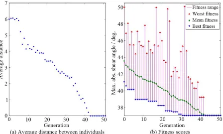
evaluating the average distance between individuals, shown in Fig. 6a. For the first six

generations the value is approximately 6, indicating that the initial population covers

approximately 70 % (6/8.7) of the solution space. The average distance reduces by 1.6 %

(0.14/761/2) for each subsequent generation, indicating that evolution is progressive,

allowing sufficient opportunity for elite genes, (i.e. genes related to low fitness scores in

terms of maximum shear angles), to survive during offspring creation.

Fig. 6b shows the evolution of the fitness scores for Step I. The magnitude of the adaptive

Fitness Range is similar for each generation until the Best Fitness converges, implying

that a wide search range has been adopted throughout. The range of the fitness score

varies due to adaptive mutation. The optimum solution (i.e. convergence of the Best

Fitness) is achieved during generation 31. Perturbations induced by further mutations

during the next 12 generations (indicated by a non-zero fitness range) appear to have no

influence on the optimal solution. Furthermore, the mutation probability reduces to zero

following generation 43, after the optimal solution has been determined. Therefore, Fig.

6 confirms that the present diversity prevents local optimum solutions, random selection

and instability.

The maximum shear angle decreases by 11.2, from 48.2for the fully constrained system

(Fig. 7a) to 37.1after all unconstrained springs have been removed (Fig 7b). However,

individual springs are required to obtain the blank boundary conditions. Therefore, it is

necessary to compromise and combine neighbouring clamps and eliminate isolated ones

(see Fig. 7c). The minimum threshold distance between clamps was chosen to be 25 mm

(equivalent to the width of 5 finite elements), and the minimum clamp length was also

assumed to be 25 mm. In addition, the spring located at the mid-point of the short edge

(see Fig. 7b) was removed, as this could not be combined into a single clamp due to the

region of high curvature generated by the springs either side. Consequently, only two

clamps were required along each of the short edges to maintain the optimum draw-in. The

individual constrained positions from Fig. 7b were combined and reduced to 14 clamps,

as shown in Fig 7c. The stiffness of each consolidated spring was directly obtained by

summing the stiffness of all of the parallel springs belonging to each corresponding block.

Table 2 provides a summary of the spring stiffnesses after Step I of the optimisation,

including the length and position of the corresponding clamps.

Although the maximum shear angle increased by 3.4in Fig. 7c compared with the result

in Fig. 7b, this still yields an overall reduction in peak shear angle of 7.7compared with

the unoptimised case. In addition, the shear angle distribution in Fig. 7b indicates that

wrinkling occurs along the long edges when constrained by individual springs, as there

are local transitions in shear angle. However, these disappear in Fig. 7c when longer

clamps are introduced along the edges. Constraining the blank using consolidated clamps

homogenises the boundary constraints to eliminate undesirable wrinkling around the

4.2 Stiffness optimisation from Step II

The spring stiffnesses from the solution in Step I (Fig. 7c) form the starting point of Step

II. Half of the individuals for the zeroth generation used the same combination of

constraint properties as the solution from Step I and the rest were generated randomly,

which then evolved into subsequent generations according to the GA. The population size

for the GA was 20 in each generation, and the tolerance for the fitness function was 0.05°.

For the current work, the range of spring stiffnesses in this step was chosen to be from

0.03 N/mm to 0.50 N/mm. The stability of the optimisation for Step II was validated using

the same methodology outlined for Step I. The fitness scores confirmed that the initial

population was suitably diverse, and Fig. 8a indicates that the solution was stable.

As shown in Fig. 8a, the maximum shear angle is reduced to 37.2 by optimising the

spring stiffnesses. This value differs by 0.1from the ideal optimum (37.1) in Step I (see

in Fig. 7b). It indicates that the negative influence induced by artificially adjusting the

constrained positions is minimised by seeking an optimal combination of clamp

stiffnesses in Step II, whilst making the solution more practical. Comparison of the

maximum shear angles during each step therefore confirms that the two-stage

optimisation does not significantly compromise the optimisation outcome. Using a more

generic GA approach may enable both optimisation stages to be combined (e.g. assigning

different sets of genes defining positions and stiffnesses) to further improve the accuracy

of the solution. However, this would require variable encoding lengths to be used for the

different parameters. Encoding the task as a single step optimisation problem may result

in a more efficient solution in the longer term, but it would be more complex to implement

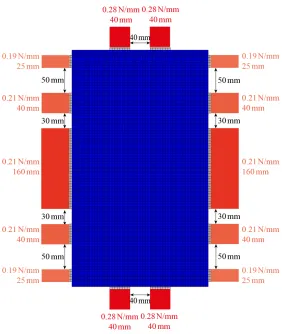
The convergence of the spring stiffnesses for Step II is presented in Fig. 8b. The optimum

combination of spring stiffnesses is presented in Table 2 and illustrated schematically in

Fig. 9. This figure allows a general strategy for spring placement to be derived: At zones

of the component geometry with small curvature, springs with relatively low stiffness are

attached through long clamps to provide near uni-axial tension. Zones with a high degree

of curvature require multiple springs with stiffnesses adapted to suit the fibre orientation,

which are attached through short localised clamps, allowing for multi-axial tension to be

applied to the blank. In general, springs attached to the clamps along the long edges have

a stiffness of 0.20 N/mm, and springs along the short edges are approximately 0.30 N/mm

for the current geometry. These are of similar magnitude to those used by Harrison et al.

[13], where fewer clamps were used, and the stiffer springs were placed on the long edges.

Figure 10 illustrates in-plane strains along the two principal fibre directions, where only

negative strains are shown. These negative strains indicate fabric compression, which

may result in localised wrinkles. The progression of the images implies that maximum

strains along both fibre orientations have been reduced through strain homogenisation

during optimisation, resulting in a reduction of potential regions of severe wrinkling.

Whilst the shear angle distribution was the optimisation objective, the distribution of

wrinkling strain is simultaneously homogenised as previously seen in a recent study [15].

5 Conclusions

A scenario has been introduced for controlling material draw-in during reinforcement

forming processes, using a series of in-plane springs to locally apply tension to the

preform, rather than using a blank holder to compress the preform out-of-plane and apply

bi-axial materials with large deformation, based on a VFABRIC model in

Abaqus/Explicit. The in-plane constraints around the edges were modelled using spring

elements connected to a fully constrained rigid frame, providing axial forces to control

material slippage into the cavity.

An optimisation methodology has been developed by combining the explicit FE model

with a genetic algorithm to optimise parameters associated with the in-plane constraints.

It has been implemented in two stages: (a) Step I: Clamping arrangement optimisation,

(b) Step II: Spring stiffness Optimisation. Process optimisation has been demonstrated

using a double-dome geometry from the literature. Results indicate that controlling

material draw-in by constraining the blank in-plane around the perimeter is an effective

way of homogenising the global shear angle distribution and minimising the local

maximum value. The peak shear angle was reduced from 48.2 to 37.2 following the

two-stage optimisation process. Strains along the two principal fibre directions have also

been reduced during the optimisation, through strain homogenisation, resulting in a

reduction of potential regions of severe wrinkling.

Acknowledgements

The work presented in this paper was completed as part of the “Affordable

Lightweighting Through Pre-form Automation” (ALPA) project. The authors gratefully

acknowledge the financial support of the Technology Strategy Board and technical

support from the project partners: McLaren Automotive, Formax, the Advanced

References

[1] Long AC, Clifford MJ. Composite forming mechanisms and materials characterisation. In: Long AC,

editor.Composite forming technologies. Cambridge: Woodhead Publishing Ltd., 2007. p. 1-21.

[2] Lin H, Wang J, Long AC, Clifford MJ, Harrison P. Predictive modelling for optimization of textile

composite forming. Compos Sci Technol2007; 67(15–16): 3242-3252.

[3] Yu WR, Harrison P, Long AC. Finite element forming simulation for crimp fabrics using a

non-orthogonal constitutive equation.Compos Part A-Appl S2005; 36(8): 1079-1093.

[4] Van Der Weeën F. Algorithms for draping fabrics on doubly-curved surfaces.Int J Numer Meth Eng

1991; 31(7): 1415-1426.

[5] Skordos AA, Sutcliffe MP, Klintworth JW, Adolfsson P. Multi-objective optimisation of woven

composite draping using genetic algorithms. In:27th International Conference SAMPE Europe. Paris,

2006.

[6] Yu WR, Pourboghrat F, Chung K, Zampaloni M, Kang TJ. Non-orthogonal constitutive equation for

woven fabric reinforced thermoplastic composites.Compos Part A-Appl S2002; 33(8): 1095-1105.

[7] Xue P, Peng X, Cao J. A non-orthogonal constitutive model for characterizing woven composites.

Compos Part A-Appl S2003; 34(2): 183-193.

[8] Wei L, Yuying Y. Multi-objective optimization of sheet metal forming process using Pareto-based

genetic algorithm.J Mater Process Tech2008; 208(1–3): 499-506.

[9] Conceição António CA, Magalhães Dourado N. Metal-forming process optimisation by inverse

evolutionary search.J Mater Process Tech2002; 121(2–3): 403-413.

[10] Chung JS, Hwang SM. Application of a genetic algorithm to process optimal design in non-isothermal

metal forming.J Mater Process Tech1998; 80–81: 136-143.

[11] Kahhal P, Brooghani S, Azodi H. Multi-objective Optimization of Sheet Metal Forming Die Using

Genetic Algorithm Coupled with RSM and FEA.Journal of Failure Analysis and Prevention 2013;

13(6): 771-778.

[12] Skordos AA, Aceves CM, Sutcliffe MPF. Drape optimisation in woven composite manufacturing. In:

5th International Conference on Inverse Problems in Engineering: Theory and Practice. Cambridge,

2005.

[13] Harrison P, Gomes R, Curado-Correia N. Press forming a 0/90 cross-ply advanced thermoplastic

composite using the double-dome benchmark geometry.Compos Part A-Appl S2013; 54: 56-69.

[14] Willems A. Forming simulation of textile reinforced composite shell structures. PhD dissertation,

Katholieke Universiteit Leuven, 2008.

[15] Chen S, Endruweit A, Harper LT, Warrior NA. Inter-ply stitching optimisation of highly drapeable

multi-ply preforms.Compos Part A-Appl S2015; 71: 144-156.

[16] Peng X, Cao J. A dual homogenization and finite element approach for material characterization of

textile composites.Compos Part B-Eng2002; 33(1): 45-56.

[17] Peng X, Cao J. A continuum mechanics-based non-orthogonal constitutive model for woven

[18] Harrison P, Gomes R, Correia N, Abdiwi F, Yu WR. Press forming the double-dome benchmark

geometry using a 0/90 uniaxial cross-ply advanced thermoplastic composite. In: 15th European

Conference on Composite Materials. Venice, 2012.

[19] Khan MA. Numerical and Experimental Forming Analyses of Textile Composite Reiforcements

Based on a Hypoelastic Behaviour. PhD dissertation, Institut National des Sciences Appliquees de

Lyon, 2009.

[20] Khan MA, Mabrouki T, Vidal-Sallé E, Boisse P. Numerical and experimental analyses of woven

composite reinforcement forming using a hypoelastic behaviour. Application to the double dome

benchmark.J Mater Process Tech2010; 210(2): 378-388.

[21] Cao J, Akkerman R, Boisse P, Chen J, Cheng HS, de Graaf EF, Gorczyca JL, Harrison P, Hivet G,

Launay J, Lee W, Liu L, Lomov SV, Long A, de Luycker E, Morestin F, Padvoiskis J, Peng XQ,

Sherwood J, Stoilova Tz, Tao XM, Verpoest I, Willems A, Wiggers J, Yu TX, Zhu B.

Characterization of mechanical behavior of woven fabrics: experimental methods and benchmark

results.Compos Part A-Appl S2008; 39(6): 1037-1053.

[22] Peng X, Rehman ZU. Textile composite double dome stamping simulation using a non-orthogonal

Tables

Table 1.Comparison of shear angle data from Abaqus/Explicit VFABRIC model against two sets of experimental results from literature [14].

ID

coord. (mm) shear angle (deg.)

ID

coord. (mm) shear angle (deg.)

x y

exp.

(case 1)

exp.

(case 2)

num. x y

exp.

(case 1)

exp.

(case 2)

num.

1 85 65 4.4 ± 2.9 3.3 ± 0.8 2.0 11 17.3 202.7 7.6 ± 1.5 6.2 ± 1.9 7.8

2 60 40 0.1 ± 0.5 0.1 ± 0.4 0.3 12 26 188 14.1 ± 0.7 13.7 ± 1.1 14.3

3 45 40 0.3 ± 0.3 0.3 ± 0.5 0.4 13 34.7 171.8 14.5 ± 2.1 15.2 ± 0.7 15.6

4 10 40 -0.4 ± 1.1 0.5 ± 1.1 0.7 14 44.6 155.9 22.3 ± 2.4 23.3 ± 1.9 25.0

5 60 80 3.7 ± 1.4 3.0 ± 2.0 2.8 15 52 142.1 31.5 ± 2.3 32.1 ± 2.1 32.8

6 45 80 0.5 ± 1.3 -0.5 ± 1.6 1.4 16 60 127.6 29.2 ± 1.8 29.1 ± 1.3 31.0

7 10 80 1.4 ± 1.4 -0.9 ± 0.9 2.7 17 68.9 112.6 15.8 ± 1.5 12.7 ± 3.0 12.1

8 25 120 11.9 ± 1.2 14.0 ± 2.1 12.1 18 77.1 97.2 4.0 ± 0.6 2.1 ± 2.7 4.7

9 5 140 7.0 ± 1.1 6.9 ± 0.4 7.0 19 84.9 83.4 4.1 ± 1.1 1.3 ± 2.9 5.0

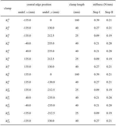
Table 2.Clamping parameters obtained from Step I and Step II (The origin of the undeformed coordinate

system is the centre of the blank).

clamp

central edge position clamp length stiffness (N/mm)

undef.x(mm) undef.y(mm) (mm) Step I Step II

݇ଵ௖௧ -135.0 0 160 0.39 0.21

݇ଶ௖௧ -135.0 130.0 40 0.27 0.21

݇ଷ௖௧ -135.0 212.5 25 0.09 0.19

݇ସ௖௧ -40.0 235.0 40 0.21 0.28

݇ହ௖௧ 40.0 235.0 40 0.21 0.28

݇଺௖௧ 135.0 212.5 25 0.09 0.19

݇଻௖௧ 135.0 130.0 40 0.27 0.21

଼݇௖௧ 135.0 0 160 0.39 0.21

݇ଽ௖௧ 135.0 -130.0 40 0.27 0.21

݇ଵ଴௖௧ 135.0 -212.5 25 0.09 0.19

݇ଵଵ௖௧ 40.0 -235.0 40 0.21 0.28

݇ଵଶ௖௧ -40.0 -235.0 40 0.21 0.28

݇ଵଷ௖௧ -135.0 -212.5 25 0.09 0.19

Figures

Fig. 1.Comparison of fabric forming model using in-plane constraints against experimental results from literature [14]; fibre orientation is 0°/90°.

Fig. 4.Implementation of Step II - Near-optimisation of constraint properties.

Fig. 6.(a) Population diversity and (b) optimisation evolution for Step I.