Learning Concept Taxonomies from Multi modal Data

Learning Concept Taxonomies from Multi-modal Data

Hao Zhang1_{, Zhiting Hu}1_{, Yuntian Deng}1_{, Mrinmaya Sachan}1_,

Zhicheng Yan2_{, Eric P. Xing}1 1_{Carnegie Mellon University,}2_UIUC

{hao,zhitingh,yuntiand,mrinmays,epxing}@cs.cmu.edu

Abstract

We study the problem of automatically building hypernym taxonomies from tex-tual and visual data. Previous works in taxonomy induction generally ignore the increasingly prominent visual data, which encode important perceptual semantics. Instead, we propose a probabilistic model for taxonomy induction by jointly leverag-ing text and images. To avoid hand-crafted feature engineering, we design end-to-end features based on distributed representa-tions of images and words. The model is discriminatively trained given a small set of existing ontologies and is capable of building full taxonomies from scratch for a collection of unseen conceptual label items with associated images. We evalu-ate our model and features on the WordNet hierarchies, where our system outperforms previous approaches by a large gap.

1 Introduction

Human knowledge is naturally organized as se-mantic hierarchies. For example, in WordNet (Miller, 1995), specific concepts are categorized and assigned to more general ones, leading to a semantic hierarchical structure (a.k.a taxonomy). A variety of NLP tasks, such as question answer-ing (Harabagiu et al., 2003), document cluster-ing (Hotho et al., 2002) and text generation (Biran and McKeown, 2013) can benefit from the con-ceptual relationship present in these hierarchies.

Traditional methods of manually constructing taxonomies by experts (e.g. WordNet) and interest communities (e.g. Wikipedia) are either knowl-edge or time intensive, and the results have lim-ited coverage. Therefore, automatic induction of taxonomies is drawing increasing attention in both

(a) Input

Seafish

Shark Ray

Seafish

Ray Shark

“seafish, such as sharksand rays…” “sharkand rayare a group of seafish…” “either rayor sharklives in …”

(b) Output

visual similarity wordvec closeness

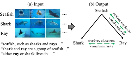
Figure 1: An overview of our system. (a) Input: a collection of label items, represented by text and images; (b) Output: we build a taxonomy from scratch by extracting features based on distributed representations of text and images.

NLP and computer vision. On one hand, a num-ber of methods have been developed to build hi-erarchies based on lexical patterns in text (Yang and Callan, 2009; Snow et al., 2006; Kozareva and Hovy, 2010; Navigli et al., 2011; Fu et al., 2014; Bansal et al., 2014; Tuan et al., 2015). These works generally ignore the rich visual data which encode important perceptual semantics (Bruni et al., 2014) and have proven to be complemen-tary to linguistic information and helpful for many tasks (Silberer and Lapata, 2014; Kiela and Bot-tou, 2014; Zhang et al., 2015; Chen et al., 2013). On the other hand, researchers have built visual hi-erarchies by utilizing only visual features (Griffin and Perona, 2008; Yan et al., 2015; Sivic et al., 2008). The resulting hierarchies are limited in in-terpretability and usability for knowledge transfer. Hence, we propose to combine both visual and textual knowledge to automatically build tax-onomies. We induce is-a taxonomies by su-pervised learning from existing entity ontologies where each concept category (entity) is associated with images, either from existing dataset (e.g. Im-ageNet (Deng et al., 2009)) or retrieved from the web using search engines, as illustrated in Fig 1. Such a scenario is realistic and can be extended to a variety of tasks; for example, in knowledge base

construction (Chen et al., 2013), text and image collections are readily available but label relations among categories are to be uncovered. In large-scale object recognition, automatically learning relations between labels can be quite useful (Deng et al., 2014; Zhao et al., 2011).

Both textual and visual information provide im-portant cues for taxonomy induction. Fig 1 il-lustrates this via an example. The parent cate-gory seafish and its two child categories shark and ray are closely related as: (1) there is a hypernym-hyponym (is-a) relation between the words “seafish” and “shark”/“ray” through text de-scriptions like “...seafish, such as shark and ray...”, “...shark and ray are a group of seafish...”; (2) images of the close neighbors, e.g., shark and ray are usually visually similar and images of the child, e.g. shark/ray are similar to a sub-set of images of seafish. To effectively capture these patterns, in contrast to previous works that rely on various hand-crafted features (Chen et al., 2013; Bansal et al., 2014), we extract features by leveraging thedistributed representationsthat em-bed images (Simonyan and Zisserman, 2014) and words (Mikolov et al., 2013) as compact vectors, based on which the semantic closeness is directly measured in vector space. Further, we develop a probabilistic framework that integrates the rich multi-modal features to induce “is-a” relations be-tween categories, encouraginglocal semantic con-sistencythat each category should be visually and textually close to its parent and siblings.

In summary, this paper has the following con-tributions: (1) We propose a novel probabilistic Bayesian model (Section 3) for taxonomy induc-tion by jointly leveraging textual and visual data. The model is discriminatively trained and can be directly applied to build a taxonomy from scratch for a collection of semantic labels. (2) We de-sign novel features (Section 4) based on general-purpose distributed representations of text and im-ages to capture both textual and visual relations between labels. (3) We evaluate our model and features on the ImageNet hierarchies with two dif-ferent taxonomy induction tasks (Section 5). We achieve superior performance on both tasks and improve theF1 score by 2x in thetaxonomy con-struction task, compared to previous approaches. Extensive comparisons demonstrate the effective-ness of integrating visual features with language features for taxonomy induction. We also provide

qualitative analysis on our features, the learned model, and the taxonomies induced to provide fur-ther insights (Section 5.3).

2 Related Work

Many approaches have been recently developed that build hierarchies purely by identifying either lexical patterns or statistical features in text cor-pora (Yang and Callan, 2009; Snow et al., 2006; Kozareva and Hovy, 2010; Navigli et al., 2011; Zhu et al., 2013; Fu et al., 2014; Bansal et al., 2014; Tuan et al., 2014; Tuan et al., 2015; Kiela et al., 2015). The approaches in Yang and Callan (2009) and Snow et al. (2006) assume a starting incomplete hierarchy and try to extend it by in-serting new terms. Kozareva and Hovy (2010) and Navigli et al. (2011) first find leaf nodes and then use lexical patterns to find intermediate terms and all the attested hypernymy links between them. In (Tuan et al., 2014), syntactic contextual similarity is exploited to construct the taxonomy, while Tuan et al. (2015) go one step further to consider trusti-ness and collective synonym/contrastive evidence. Different from them, our model is discriminatively trained with multi-modal data. The works of Fu et al. (2014) and Bansal et al. (2014) use similar language-based features as ours. Specifically, in (Fu et al., 2014), linguistic regularities between pretrained word vectors (Mikolov et al., 2013) are modeled as projection mappings. The trained projection matrix is then used to induce pairwise hypernym-hyponym relations between words. Our features are partially motivated by Fu et al. (2014), but we jointly leverage both textual and visual in-formation. In Kiela et al. (2015), both textual and visual evidences are exploited to detect pairwise lexical entailments. Our work is significantly dif-ferent as our model is optimized over the whole taxonomy space rather than considering only word pairs separately. In (Bansal et al., 2014), a struc-tural learning model is developed to induce a glob-ally optimal hierarchy. Compared with this work, we exploit much richer features from both text and images, and leverage distributed representations instead of hand-crafted features.

In (Griffin and Perona, 2008) and (Marszałek and Schmid, 2008), a visual taxonomy is built to ac-celerate image categorization. In (Chen et al., 2013), only binary object-object relations are ex-tracted using co-detection matrices. Our work dif-fers from all of these as we integrate textual with visual information to construct taxonomies.

Also of note are several works that integrate text and images as evidence for knowledge base autocompletion (Bordes et al., 2011) and zero-shot recognition (Gan et al., 2015; Gan et al., ; Socher et al., 2013). Our work is different be-cause our task is to accurately construct multi-level hyponym-hypernym hierarchies from a set of (seen or unseen) categories.

3 Taxonomy Induction Model

Our model is motivated by the key observation that in a semantically meaningful taxonomy, a cate-gory tends to be closely related to its children as well as its siblings. For instance, there exists a hypernym-hyponym relation between the name of categoryshark and that of its parentseafish. Be-sides, images of shark tend to be visually simi-lar to those of ray, both of which are seafishes. Our model is thus designed to encourage such lo-cal semantic consistency; and by jointly consider-ing all categories in the inference, a globally opti-mal structure is achieved. A key advantage of the model is that we incorporate both visual and tex-tual features induced from distributed representa-tions of images and text (Section 4). These fea-tures capture the rich underlying semantics and facilitate taxonomy induction. We further distin-guish the relative importance of visual and tex-tual features that could vary in different layers of a taxonomy. Intuitively, visual features would be increasingly indicative in the deeper layers, as sub-categories under the same category of specific objects tend to be visually similar. In contrast, textual features would be more important when inducing hierarchical relations between the cate-gories of general concepts (i.e. in the near-root layers) where visual characteristics are not neces-sarily similar.

3.1 The Problem

Assume a set of N categories x = {x1, x2, . . . , xN}, where each category xn consists of a text term tn as its name, as well as a set of images in = {i1, i2, . . .}. Our goal

is to construct a taxonomy tree T over these categories1_{, such that categories of specific object} types (e.g. shark) are grouped and assigned to those of general concepts (e.g. seafish). As the categories in x may be from multiple disjoint taxonomy trees, we add apseudo category x0 as the hyper-root so that the optimal taxonomy is en-sured to be a single tree. Letzn ∈ {1, . . . , N}be the index of the parent of categoryxn, i.e. xzn is

the hypernymic category ofxn. Thus the problem of inducing a taxonomy structure is equivalent to inferring the conditional distributionp(z|x) over the set of (latent) indicesz ={z1, . . . , zn}, based on the images and text.

3.2 Model

We formulate the distribution p(z|x) through a model which leverages rich multi-modal features. Specifically, letcnbe the set of child nodes of cat-egoryxnin a taxonomy encoded byz. Our model is defined as

pw(z,π|x,α)∝p(π|α) N

Y

n=1

Y

xn0∈c_n

πngw(xn, xn0,c_n\x_n0)

(1) wheregw(xn, xn0,c_n\x_n0), defined as

gw(xn, xn0,cn\xn0) = exp{w>_d(x

n0)fn,n0_,cn\xn0},

measures the semantic consistency between cate-gory xn0, its parent x_n as well as its siblings

in-dexed by cn\xn0. The function g_w(·) is

loglin-ear with respect tof_n,n0_,cn\x

n0, which is the

fea-ture vector defined over the set of relevant cate-gories(xn, xn0,c_n\x_n0), withc_n\x_n0being the set

of child categories excludingxn0 (Section 4). The

simple exponential formulation can effectively en-courage close relations among nearby categories in the induced taxonomy. The function has com-bination weightsw ={w1, . . . ,wL}, whereLis the maximum depth of the taxonomy, to capture the importance of different features, and the func-tiond(xn0)to return the depth ofx_n0in the current

taxonomy. Each layerl(1 ≤ l ≤ L) of the tax-onomy has a specificwlthereby allowing varying weights of the same features in different layers. The parameters are learned in asupervised man-ner. In eq 1, we also introduce a weightπnfor each nodexn, in order to capture the varying popular-ity of different categories (in terms of being a par-ent category). For example, some categories like

1_{We assumeTto be a tree. Most existing taxonomies are}

plantcan have a large number of sub-categories, while others such asstonehave less. We modelπ

as a multinomial distribution with Dirichlet prior

α= (α1, . . . , αN)to encode any prior knowledge of the category popularity2_{; and the conjugacy} al-lows us to marginalize outπanalytically to get

pw(z|x,α)∝

Z

p(π|α)

N

Y

n=1

Y

xn0∈cn

πngw(xn, xn0,c_n\x_n0)dπ

∝Y

n

Γ(qn+αn) Y x_n0∈c_n

gw(xn, xn0,cn\xn0)

(2) whereqnis the number of children of categoryxn. Next, we describe our approach to infer the ex-pectation for each zn, and based on that select a particular taxonomy structure for the category nodesx. Aszis constrained to be a tree (i.e. cycle without loops), we include with eq 2, an indicator factor1(z)that takes1ifzcorresponds a tree and 0 otherwise. We modify the inference algorithm appropriately to incorporate this constraint. Inference. Exact inference is computationally in-tractable due to the normalization constant of eq 2. We therefore use Gibbs Sampling, a procedure for approximate inference. Here we present the sam-pling formula for each zn directly, and defer the details to the supplementary material. The sam-pling procedure is highly efficient because the nor-malization term and the factors that are irrelevant toznare cancelled out. The formula is

p(zn=m|z\zn,·)∝1(zn=m,z\zn)· q−mn+αm·

Q

x_n0∈cm∪{xn}gw(xm, xn0,cm∪ {xn}) Q

x_n0∈cm\xngw(xm, xn0,cm\xn)

,

(3) where qm is the number of children of category

m; the superscript−ndenotes the number exclud-ing xn. Examining the validity of the taxonomy structure (i.e. the tree indicator) in each sampling step can be computationally prohibitive. To han-dle this, we restrict the candidate value of zn in eq 3, ensuring that the new zn is always a tree. Specifically, given a treeT, we define astructure operationas the procedure of detaching one node

xninT from its parent and appending it to another nodexmwhich is not a descendant ofxn.

Proposition 1. (1) Applying a structure operation on a tree T will result in a structure that is still a tree. (2) Any tree structure over the node setx

that has the same root node with tree T can be achieved by applying structure operation on T a finite number of times.

2_{αcould be estimated using training data.}

The proof is straightforward and we omit it due to space limitations. We also add a pseudo node

x0 as the fixed root of the taxonomy. Hence by initializing a tree-structured state rooted atx0 and restricting each updating step as a structure opera-tion, our sampling procedure is able to explore the whole valid tree space.

Output taxonomy selection. To apply the model to discover the underlying taxonomy from a given set of categories, we first obtain the marginals ofz

by averaging over the samples generated through eq 3, then output the optimal taxonomyz∗_by find-ing the maximum spannfind-ing tree (MST) usfind-ing the Chu-Liu-Edmonds algorithm (Chu and Liu, 1965; Bansal et al., 2014).

Training. We need to learn the model parame-ters wl of each layer l, which capture the rela-tive importance of different features. The model is trained using the EM algorithm. Let `(xn) be the depth (layer) of category xn; and ˜z (siblings ˜

cn) denote the gold structure in training data. Our training algorithm updates w through maximum likelihood estimation, wherein the gradient ofwl is (see the supplementary materials for details):

δw_l= X

n:`(xn)=l

{f(x_z˜n, x_n,˜c_n\x_n)−E_p[f(x_zn, x_n,c_n\x_n)]},

which is the net difference between gold feature vectors and expected feature vectors as per the model. The expectation is approximated by col-lecting samples using the sampler described above and averaging them.

4 Features

In this section, we describe the feature vector f

al., 2013) which is widely used in diverse NLP ap-plications too. Then we designf(xn, xn0,c_n\x_n0)

based on the above image and text representations. The feature vectorf is used to measure the local semantic consistency between categoryxn0 and its

parent categoryxnas well as its siblingscn\xn0.

4.1 Image Features

Sibling similarity. As mentioned above, close neighbors in a taxonomy tend to be visually simi-lar, indicating that the embedding of images of sib-ling categories should be close to each other in the vector spaceRa_{. For a categoryx}

nand its image setin, we fit a Gaussian distributionN(vin,Σn)

to the image vectors, wherevin ∈Rais the mean

vector andΣn ∈ Ra×a is the covariance matrix. For a sibling categoryxmofxn, we define the vi-sual similarity betweenxnandxmas

vissim(xn, xm)=[N(vim;vin,Σn)+N(vin;vim,Σm)]/2

which is the average probability of the mean im-age vector of one category under the Gaussian dis-tribution of the other. This takes into account not only the distance between the mean images, but also the closeness of the images of each category. Accordingly, we compute the visual similarity be-tweenxn0 and the setc_n\x_n0 by averaging:

vissim(xn0,cn\xn0) = P

xm∈cn\xn0vissim(xn0, xm)

|c_n| −1 . We then bin the values of vissim(xn0,c_n\x_n0)

and represent it as an one-hot vector, which consti-tutesf as a component named assiblings image-image relation feature(denoted asS-V13_).

Parent prediction. Similar to feature S-V1, we also create the similarity feature between the im-age vectors of the parent and child, to measure their visual similarity. However, the parent node is usually a more general concept than the child, and it usually consists of images that are not necessar-ily similar to its child. Intuitively, by narrowing the set of images to those that are most similar to its child improves the feature. Therefore, different from S-V1, when estimating the Gaussian distri-bution of the parent node, we only use the topK

images with highest probabilities under the Gaus-sian distribution of the child node. We empirically show in section 5.3 that choosing an appropriate

K consistently boosts the performance. We name this feature as parent-child image-image relation feature(denoted asPC-V1).

3_{S: sibling, PC: parent-child, V: visual, T: textual.}

Further, inspired by the linguistic regularities of word embedding, i.e. the hypernym-hyponym re-lationship between words can be approximated by a linear projection operator between word vectors (Mikolov et al., 2013; Fu et al., 2014), we design a similar strategy to (Fu et al., 2014) between im-ages and words so that the parent can be “pre-dicted” given the image embedding of its child category and the projection matrix. Specifically, let(xn, xn0)be a parent-child pair in the training

data, we learn a projection matrixΦwhich min-imizes the distance betweenΦvi_n0 (i.e. the

pro-jected mean image vector vi_n0 of the child) and vtn (i.e. the word embedding of the parent):

Φ∗= argmin

Φ

1 N

X

n

kΦvi_n0 −vtnk22+λkΦk1,

whereNis the number of parent-child pairs in the training data. Once the projection matrix has been learned, the similarity between a child node xn0

and its parentxn is computed askΦvi_n0 −vtnk,

and we also create an one-hot vector by binning the feature value. We call this feature as parent-child image-word relation feature(PC-V2). 4.2 Word Features

We briefly introduce the text features employed. More details about the text feature extraction could be found in the supplementary material. Word embedding features.d PC-V1, We in-duce features using word vectors to measure both sibling-sibling and parent-child closeness in text domain (Fu et al., 2014). One exception is that, as each category has only one word, the sibling sim-ilarity is computed as the cosine distance between two word vectors (instead of mean vectors). This will produce another two parts of features, parent-child word-word relation feature(PC-T1) and sib-lings word-word relation feature(S-T1).

Word surface features. In addition to the embedding-based features, we further leverage lexical features based on the surface forms of child/parent category names. Specifically, we employ the Capitalization, Ends with, Contains, Suffix match, LCS and Length different features, which are commonly used in previous works in taxonomy induction (Yang and Callan, 2009; Bansal et al., 2014).

5 Experiments

bet-ter reproducibility. We then compare our model with previous state-of-the-art methods (Fu et al., 2014; Bansal et al., 2014) with two taxonomy in-duction tasks. Finally, we provide analysis on the weights and taxonomies induced.

5.1 Implementation Details

Dataset. We conduct our experiments on the Im-ageNet2011 dataset (Deng et al., 2009), which provides a large collection of category items (synsets), with associated images and a label hi-erarchy (sampled from WordNet) over them. The original ImageNet taxonomy is preprocessed, re-sulting in a tree structure with 28231 nodes. Word embedding training. We train word em-bedding for synsets by replacing each word/phrase in a synset with a unique token and then us-ing Google’s word2vec tool (Mikolov et al., 2013). We combine three public available cor-pora together, including the latest Wikipedia dump (Wikipedia, 2014), the One Billion Word Lan-guage Modeling Benchmark (Chelba et al., 2013) and the UMBC webbase corpus (Han et al., 2013), resulting in a corpus with total 6 billion tokens. The dimension of the embedding is set to200. Image processing. we employ the ILSVRC12 pre-trained convolutional neural networks (Si-monyan and Zisserman, 2014) to embed each im-age into the vector space. Then, for each category

xnwith images, we estimate a multivariate Gaus-sian parameterized by Nxn = (µxn,Σxn), and

constrainΣxnto be diagonal to prevent overfitting.

For categories with very few images, we only es-timate a mean vectorµxn. For nodes that do not

have images, we ignore the visual feature.

Training configuration. The feature vector is a concatenation of 6 parts, as detailed in section 4. All pairwise distances are precomputed and stored in memory to accelerate Gibbs sampling. The ini-tial learning rate for gradient descent in the M step is set to 0.1, and is decreased by a fraction of 10 every 100 EM iterations.

5.2 Evaluation

5.2.1 Experimental Settings

We evaluate our model on three subtrees sampled from the ImageNet taxonomy. To collect the sub-trees, we start from a given root (e.g. consumer goods) and traverse the full taxonomy using BFS, and collect all descendant nodes within a depthh

(number of nodes in the longest path). We varyh

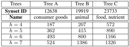
Trees Tree A Tree B Tree C

Synset ID 12638 19919 23733

Name consumer goods animal food, nutrient

h= 4 187 207 572 h= 5 362 415 890 h= 6 493 800 1166 h= 7 524 1386 1326

Table 1: Statistics of our evaluation set. The bot-tom 4 rows give the number of nodes within each height h ∈ {4,5,6,7}. The scale of the threes range from small to large, and there is no overlap-ping among them.

to get a series of subtrees with increasing heights

h ∈ {4,5,6,7} and various scales (maximally 1326 nodes) in different domains. The statistics of the evaluation sets are provided in Table 1. To avoid ambiguity, all nodes used in ILSVRC 2012 are removed as the CNN feature extractor is trained on them.

We design two different tasks to evaluate our model. (1) In the hierarchy completion task, we randomly remove some nodes from a tree and use the remaining hierarchy for training. In the test phase, we infer the parent of each removed node and compare it with groundtruth. This task is de-signed to figure out whether our model can suc-cessfully induce hierarchical relations after learn-ing from within-domain parent-child pairs. (2) Different from the previous one, the hierarchy construction task is designed to test the gener-alization ability of our model, i.e. whether our model can learn statistical patterns from one hi-erarchy and transfer the knowledge to build a tax-onomy for another collection of out-of-domain la-bels. Specifically, we select two trees as the train-ing set to learnw. In the test phase, the model is required to build the full taxonomy from scratch for the third tree.

We use Ancestor F1 as our evaluation metric (Kozareva and Hovy, 2010; Navigli et al., 2011; Bansal et al., 2014). Specifically, we measure

F1 = 2P R/(P+R)values of predicted “is-a” re-lations where the precision (P) and recall (R) are:

P =|isapredicted∩isagold|

|_isapredicted| , R=

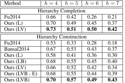
Method h= 4 h= 5 h= 6 h= 7 Hierarchy Completion

Fu2014 0.66 0.42 0.26 0.21

Ours (L) 0.70 0.49 0.45 0.37

Ours (LV) 0.73 0.51 0.50 0.42

Hierarchy Construction

Fu2014 0.53 0.33 0.28 0.18

Bansal2014 0.67 0.53 0.43 0.37

Ours (L) 0.58 0.41 0.36 0.30

Ours (LB) 0.68 0.55 0.45 0.40 Ours (LV) 0.66 0.52 0.42 0.34 Ours (LVB - E) 0.68 0.55 0.44 0.39 Ours (LVB) 0.70 0.57 0.49 0.43 Table 2: Comparisons among different variants of our model, Fu et al. (2014) and Bansal et al. (2014) on two tasks. The ancestor-F1scores are reported.

5.2.2 Results

Hierarchy completion. In thehierarchy comple-tion task, we split each tree into 70% nodes for training and 30% for test, and experiment with differenth. We compare the following three sys-tems: (1)Fu20144_{(Fu et al., 2014); (2)Ours (L):} Our model with only language features enabled (i.e. surface features, parent-child word-word re-lation feature and siblings word-word rere-lation fea-ture); (3) Ours (LV): Our model with both lan-guage features and visual features 5_{. The} aver-age performance on three trees are reported at Ta-ble 2. We observe that the performance gradu-ally drops when h increases, as more nodes are inserted when the tree grows higher, leading to a more complex and difficult taxonomy to be ac-curately constructed. Overall, our model outper-forms Fu2014 in terms of theF1score, even with-out visual features. In the most difficult case with

h = 7, our model still holds anF1 score of 0.42 (2×of Fu2014), demonstrating the superiority of our model.

Hierarchy construction.The hierarchy construc-tion task is much more difficult than hierarchy completion task because we need to build a taxon-omy from scratch given only a hyper-root. For this task, we use a leave-one-out strategy, i.e. we train our model on every two trees and test on the third, and report the average performance in Table 2. We compare the following methods: (1) Fu2014, (2) Ours (L), and (3)Ours (LV), as described above; (4)Bansal2014: The model by Bansal et al. (2014)

4_{We tried different parameter settings for the number of}

clustersCand the identification thresholdδ, and reported the best performance we achieved.

5_{In the comparisons to (Fu et al., 2014) and (Bansal et}

al., 2014), we simply setK = ∞,i.e. we use all available images of the parent category to estimate the PC-V1 feature.

retrained using our dataset; (5)Ours (LB): By ex-cluding visual features, but inex-cluding other lan-guage features from Bansal et al. (2014); (6)Ours (LVB): Our full model further enhanced with all semantic features from Bansal et al. (2014); (7) Ours (LVB - E): By excluding word embedding-based language features fromOurs (LVB).

As shown, on the hierarchy construction task, our model with only language features still outper-forms Fu2014 with a large gap (0.30compared to 0.18whenh= 7), which uses similar embedding-based features. The potential reasons are two-fold. First, we take into account not only parent-child relations but also siblings. Second, their method is designed to induce only pairwise relations. To build the full taxonomy, they first identify all pos-sible pairwise relations using a simple threshold-ing strategy and then eliminate conflicted relations to obtain a legitimate tree hierarchy. In contrast, our model is optimized over the full space of all legitimate taxonomies by taking thestructure op-erationin account during Gibbs sampling.

When comparing to Bansal2014, our model with only word embedding-based features under-performs theirs. However, when introducing vi-sual features, our performance is comparable (p-value = 0.058).Furthermore, if we discard visual features but add semantic features from Bansal et al. (2014), we achieve a slight improvement of 0.02 over Bansal2014 (p-value = 0.016), which is largely attributed to the incorporation of word embedding-based features that encode high-level linguistic regularity. Finally, if we enhance our full model with all semantic features from Bansal et al. (2014), our model outperforms theirs by a gap of 0.04 (p-value <0.01), which justifies our intuition that perceptual semantics underneath vi-sual contents are quite helpful.

5.3 Qualitative Analysis

In this section, we conduct qualitative studies to investigate how and whenthe visual information helps the taxonomy induction task.

Contributions of visual features. To evaluate the contribution of each part of the visual fea-tures to the final performance, we train our model jointly with textual features and different combi-nations of visual features, and report the

show-S-V1 PC-V1 PC-V2 h = 4 h = 5 h = 6 h = 7 0.58 0.41 0.36 0.30

X 0.63 0.48 0.40 0.32

X 0.61 0.44 0.38 0.31

X 0.60 0.42 0.37 0.31

X X 0.65 0.52 0.41 0.33

X X X 0.66 0.52 0.42 0.34

Table 3: The performance when different combi-nations of visual features are enabled.

ing that visual similarity between sibling nodes is a strong evidence for taxonomy induction. It is intuitively plausible, as it is highly likely that two specific categories share a common (and more general) parent category if similar visual contents are observed between them. Further, adding the PC-V1 feature gains us a better improvement than adding PC-V2, but both minor than S-V1.

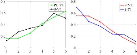
Compared to that of siblings, the visual similar-ity between parents and children does not strongly holds all the time. For example, images of Terres-trial animal are only partially similar to those of Feline, because the former one contains the later one as a subset. Our feature captures this type of “contain” relation between parents and children by considering only the top-K images from the par-ent category that have highest probabilities under the Gaussian distribution of the child category. To see this, we varyK while keep all other settings, and plot the F1 scores in Fig 2. We observe a trend that when we gradually increaseK, the per-formance goes up until reaching some maximal; It then slightly drops (or oscillates) even when more images are available, which confirms with our fea-ture design that only top images should be consid-ered in parent-child visual similarity.

Overall, the three visual features complement each other, and achieve the highest performance when combined.

Visual representations. To investigate how the image representations affect the final performance, we compare the ancestor-F1 score when differ-ent pre-trained CNNs are used for visual fea-ture extraction. Specifically, we employ both the CNN-128 model (128 dimensional feature with 15.6%top-5 error on ILSVRC12) and the VGG-16 model (4096 dimensional feature with 7.5% top-5 error) by Simonyan and Zisserman (2014), but only observe a slight improvement of 0.01 on the ancestor-F1 score for the later one.

Relevance of textual and visual features v.s. depth of tree. Compared to Bansal et al. (2014),

h = 4 h = 5

h = 6 h = 7

An

ce

ster

-F1

K /100

Figure 2: The Ancestor-F1 scores changes over K (number of images used in the PC-V1 feature) at different heights. The values in the x-axis are

K/100;K =∞means all images are used.

Figure 3: Normalized weights of each feature v.s. the layer depth.

a major difference of our model is that differ-ent layers of the taxonomy correspond to differdiffer-ent weightswl, while in (Bansal et al., 2014) all layers share the same weights. Intuitively, introducing layer-wisewnot only extends the model capacity, but also differentiates the importance of each fea-ture at different layers. For example, the images of two specific categories, such assharkandray, are very likely to be visually similar. However, when the taxonomy goes from bottom to up (spe-cific to general), the visual similarity is gradually undermined — images offishandterrestrial ani-malare not necessarily similar any more. Hence, it is necessary to privatize the weightswfor differ-ent layers to capture such variations, i.e. the visual features become more and more evident from shal-low to deep layers, while the textual counterparts, which capture more abstract concepts, relatively grow more indicative oppositely from specific to general.

correspond-millipede

invertebrate critter

animal

caterpillar domestic animal

starfish chordate

arrowworm

arthropod nematode

trichina

planarian polyp

echinoderm annelid

worm

tussock caterpillar

tent caterpillar

cephalochordate scavenger

larvacean sagitta

stocker

lancelet archiannelid

larva

foodstuff

meal, repast food, nutrient

nutriment

liquid diet

dietary

ingredient

flour grain

beef stew cows’

milk

juice water

boiled egg

barley spring

water stew

fish stew diary

product

wheat soybean

meal wheatflour brunch breakfast hard-boiled egg

water

drinking water juice

Figure 4: Excerpts of the prediction taxonomies, compared to the groundturth. Edges marked as red and green are false predictions and unpredicted groundtruth links, respectively.

ing block in wasV. Then, we average |V|and observe how its values change with the layer depth

h. For example, for the parent-child word-word relation feature, we first fetch its corresponding weightsV fromwas a20×6 matrix, where 20 is the feature dimension and 6 is the number of layers. We then average its absolute values6 _in column and get a vector v with length 6. After

`2 normalization, the magnitude of each entry in v directly reflects the relative importance of the feature as an evidence for taxonomy induction. Fig 3(b) plots how their magnitudes change with

h for every feature component averaged on three train/test splits. It is noticeable that for both word-word relations (S-T1, PC-T1), their corresponding weights slightly decrease as h increases. On the contrary, the image-image relation features (S-V1, PC-V1) grows relatively more prominent. The re-sults verify our conjecture that when the category hierarchy goes deeper into more specific classes, the visual similarity becomes relatively more in-dicative as an evidence for taxonomy induction. Visualizing results. Finally, we visualize some excerpts of our predicted taxonomies, as compared to the groundtruth in Fig 4.

6_{We take the absolute value because we only care about}

the relevance of the feature as an evidence for taxonomy in-duction, but note that the weight can either encourage (posi-tive) or discourage (nega(posi-tive) connections of two nodes.

6 Conclusion

In this paper, we study the problem of automat-ically inducing semantautomat-ically meaningful concept taxonomies from multi-modal data. We propose a probabilistic Bayesian model which leverages dis-tributed representations for images and words. We compare our model and features to previous ones on two different tasks using the ImageNet hier-archies, and demonstrate superior performance of our model, and the effectiveness of exploiting vi-sual contents for taxonomy induction. We further conduct qualitative studies and distinguish the rel-ative importance of visual and textual features in constructing various parts of a taxonomy.

Acknowledgements

We would like to thank anonymous reviewers for their valuable feedback. We would also like to thank Mohit Bansal for helpful suggestions. We thank NVIDIA for GPU donations. The work is supported by NSF Big Data IIS1447676.

References

Mohit Bansal, David Burkett, Gerard de Melo, and Dan Klein. 2014. Structured learning for taxonomy in-duction with belief propagation.

Welling. 2008. Unsupervised learning of visual tax-onomies. InCVPR.

Or Biran and Kathleen McKeown. 2013. Classifying taxonomic relations between pairs of wikipedia arti-cles.

Antoine Bordes, Jason Weston, Ronan Collobert, and Yoshua Bengio. 2011. Learning structured embed-dings of knowledge bases. InConference on Artifi-cial Intelligence, number EPFL-CONF-192344.

Elia Bruni, Nam-Khanh Tran, and Marco Baroni. 2014. Multimodal distributional semantics.

Ciprian Chelba, Tomas Mikolov, Mike Schuster, Qi Ge, Thorsten Brants, Phillipp Koehn, and Tony Robin-son. 2013. One billion word benchmark for measur-ing progress in statistical language modelmeasur-ing. arXiv preprint arXiv:1312.3005.

Xinlei Chen, Abhinav Shrivastava, and Abhinav Gupta. 2013. Neil: Extracting visual knowledge from web data. InCVPR.

Yoeng-Jin Chu and Tseng-Hong Liu. 1965. On shortest arborescence of a directed graph. Scientia Sinica.

Jia Deng, Wei Dong, Richard Socher, Li-Jia Li, Kai Li, and Li Fei-Fei. 2009. Imagenet: A large-scale hierarchical image database. InCVPR.

Jia Deng, Nan Ding, Yangqing Jia, Andrea Frome, Kevin Murphy, Samy Bengio, Yuan Li, Hartmut Neven, and Hartwig Adam. 2014. Large-scale ob-ject classification using label relation graphs. In

ECCV.

Ruiji Fu, Jiang Guo, Bing Qin, Wanxiang Che, Haifeng Wang, and Ting Liu. 2014. Learning semantic hier-archies via word embeddings. InACL.

Chuang Gan, Yi Yang, Linchao Zhu, Deli Zhao, and Yueting Zhuang. Recognizing an action using its name: A knowledge-based approach. International Journal of Computer Vision, pages 1–17.

Chuang Gan, Ming Lin, Yi Yang, Yueting Zhuang, and Alexander G Hauptmann. 2015. Exploring seman-tic inter-class relationships (SIR) for zero-shot ac-tion recogniac-tion. InAAAI.

Gregory Griffin and Pietro Perona. 2008. Learning and using taxonomies for fast visual categorization. InCVPR.

Lushan Han, Abhay Kashyap, Tim Finin, James May-field, and Jonathan Weese. 2013. Umbc ebiquity-core: Semantic textual similarity systems. Atlanta, Georgia, USA.

Sanda M Harabagiu, Steven J Maiorano, and Marius A Pasca. 2003. Open-domain textual question answer-ing techniques. Natural Language Engineering.

Andreas Hotho, Alexander Maedche, and Steffen Staab. 2002. Ontology-based text document clus-tering.

Douwe Kiela and L´eon Bottou. 2014. Learning image embeddings using convolutional neural networks for improved multi-modal semantics. InEMNLP.

Douwe Kiela, Laura Rimell, Ivan Vulic, and Stephen Clark. 2015. Exploiting image generality for lexical entailment detection. InACL.

Zornitsa Kozareva and Eduard Hovy. 2010. A semi-supervised method to learn and construct tax-onomies using the web. InEMNLP.

Marcin Marszałek and Cordelia Schmid. 2008. Con-structing category hierarchies for visual recognition. InECCV.

Tomas Mikolov, Ilya Sutskever, Kai Chen, Greg S Cor-rado, and Jeff Dean. 2013. Distributed representa-tions of words and phrases and their compositional-ity. InNIPS.

George A Miller. 1995. Wordnet: a lexical database for english. Communications of the ACM.

Roberto Navigli, Paola Velardi, and Stefano Faralli. 2011. A graph-based algorithm for inducing lexical taxonomies from scratch. InIJCAI.

Carina Silberer and Mirella Lapata. 2014. Learn-ing grounded meanLearn-ing representations with autoen-coders. InACL.

Karen Simonyan and Andrew Zisserman. 2014. Very deep convolutional networks for large-scale image recognition.arXiv preprint arXiv:1409.1556.

Josef Sivic, Bryan C Russell, Andrew Zisserman, William T Freeman, and Alexei A Efros. 2008. Un-supervised discovery of visual object class hierar-chies. InCVPR.

Rion Snow, Daniel Jurafsky, and Andrew Y Ng. 2006. Semantic taxonomy induction from heterogenous evidence. InACL.

Richard Socher, Milind Ganjoo, Christopher D Man-ning, and Andrew Ng. 2013. Zero-shot learning through cross-modal transfer. InAdvances in neural information processing systems, pages 935–943. Luu Anh Tuan, Jung-jae Kim, and Ng See Kiong.

2014. Taxonomy construction using syntactic con-textual evidence. InEMNLP.

Luu Anh Tuan, Jung-jae Kim, and Ng See Kiong. 2015. Incorporating trustiness and collective syn-onym/contrastive evidence into taxonomy construc-tion.

Zhicheng Yan, Hao Zhang, Robinson Piramuthu, Vi-gnesh Jagadeesh, Dennis DeCoste, Wei Di, and Yizhou Yu. 2015. Hd-cnn: Hierarchical deep convolutional neural networks for large scale visual recognition. InICCV.

Hui Yang and Jamie Callan. 2009. A metric-based framework for automatic taxonomy induction. In

ACL-IJCNLP.

Hao Zhang, Gunhee Kim, and Eric P. Xing. 2015. Dy-namic topic modeling for monitoring market com-petition from online text and image data. InKDD. Bin Zhao, Fei Li, and Eric P Xing. 2011. Large-scale

category structure aware image categorization. In

NIPS.