Conditional loyalty and its implications for pricing

Munich Personal RePEc Archive

Conditional loyalty and its implications

for pricing

De Francesco, Massimo A.

Department of Economics and Statistics, University of Siena (Italy)

5 November 2018

Online at

https://mpra.ub.uni-muenchen.de/91671/

Conditional loyalty and its implications for pricing

Massimo A. De Francesco

Department of Economics and statistics, University of Siena (Italy)

January 23, 2019

Abstract

Bertrand-Edgeworth competition has recently been analyzed under imperfect buyer mobility, as a game in which, once prices are chosen, a static buyer subgame (BS) is played where the buyers choose which seller to visit (see, e.g., Burdett et al, 2001). Our paper considers a symmetric duopoly where two buyers play a two-stage BS of imperfect information after price setting. With prices su¢ciently close, an equilibrium of the BS is characterized in which the buyers keep loyal if previously served. Conditional loyalty is proved to increase the …rms’ market power: at the corresponding subgame perfect equilibrium of the entire game, the price is higher than that corresponding to the equilibrium of the BS in which the buyers are persistently randomizing.

Keywords: Bertrand-Edgeworth competition, matching, imperfect buyer mobility, conditional loyalty, assessment equilibrium.

JEL Classi…cation Codes: D430, L130.

1

Introduction

Some recents contributions have addressed Bertrand-Edgeworth competition under imperfect buyer mobility, inasmuch as each buyer is allowed to visit only one seller after pricing de-cisions (Peters, 1984; Deneckere and Peck, 1995; Burdett et al., 2001; Geromichalos, 2014). Due to multiplicity of pure strategy equilibria (PSEs) of the buyer subgame (BS), price determination has been analyzed subject to the mixed strategy equilibrium (MSE) of the BS, where "mismatchings" - …rms selling below capacity along with more expensive rivals receiving positive demand - may arise.

Unlike most of this literature on pricing and "directed" search, Shi (2016) develops a multistage model where, in each stage, the …rms announce prices as well as any service priority they might o¤er to loyal buyers and the buyers, based on this information and the history of previous matchings at the various …rms, choose the probability of visiting any seller. However, even over a period in which prices remain …xed, buyers frequently seem to be able to move to another seller; furthermore, they might be uncertain as to recent capacity utilization at the various sellers. To take account of these features in the simplest way, our paper incorporates imperfect mobility into a model where two …rms, whose

total capacity equals an inelastic total demand, compete in prices and next two buyers play a two-stage BS of imperfect information, each time choosing which …rm to visit. With prices su¢ciently close to each other, two alternative equilibria of the two-stage BS are characterized. In one equilibrium, the MSE of the static BS is played repeatedly. But another equilibrium exists in which, if served, buyers keep loyal to the seller previously chosen: on the corresponding equilibrium path, both buyers are served in the second stage of the BS. Most importantly, the corresponding (subgame-perfect) equilibrium price is higher than under constant randomization.

The rest of the paper is organized as follows. To prepare the ground for our positive contribution, Section 2 analyzes duopolistic price determination when the two buyers play a static BS.2 _{Section 3 develops our model of price determination in which the two buyers}

are playing a two-stage BS of imperfect information, in each stage choosing which seller to visit. Section 4 brie‡y concludes.

2

Pricing with a static buyer subgame

Two risk-neutral …rms,A and B, sell a homogeneous commodity to two risk-neutral buyers,

h and k. (Below, notation will most often be introduced in terms of buyer h.) Each …rm

i 2 fA; Bg independently sets price pi; then a BS is played. In the static BS, any h

demands one unit if minfpA; pBg 1, 1 being each buyer’s reservation price, and chooses h, the probability of visiting A (we conveniently denote h’s strategy by h rather than h = ( h;1 h)); then eachi costlessly producesyi, the minimum between its forthcoming

demand and capacity y_i = 1. Hereafter, we take as given that

maxfpA; pBg 1: (1)

The set of possible events buyer h may experience is Eh = fehg = fAsh; Arh; Bsh; Brhg:

ish (irh) stands for h visiting i 2 fA; B] and being served (rationed). With both buyers

at i, each is served with equal probability. Denote by (eh)( h; k), uh( h; k), (Eyi)( h; k),

and (E i)( h; k) = pi(Eyi)( h; k), respectively, the probability of eh, h’s payo¤ (expected

surplus),i’s expected output and pro…t under strategy pro…le( h; k). Given k,h’s service

probability and payo¤ are (Ash)(1; k) = k

2 + 1 k and uh(1; k) = (1 pA) (Ash)(1; k),

respectively, if visiting A, and (Bsh)(0; k) = k+

1 k

2 anduh(0; k) = (1 pB) (Bsh)(0; k)

if visiting B. With pA and pB meeting system

2pB 1 pA

1 +pB

2 ; (2)

the BS has a symmetric equilibrium,( h; k) = (e;e), where buyers are indi¤erent between

the …rms: _e, the solution of

(1 pA) (Ash)(1; ) = (1 pB) (Bsh)(0; ); (3) 2_{The basic result is already in Burdett et al. (2001, pp. 1062-1067) where the two-seller two-buyer case}

equals

e=_e(pA; pB) =

1 2pA+pB

2 pA pB

: (4)

Note thatpB <1(pB = 1) is equivalent to 2pB 1< 1+₂pB <1(2pB 1 = 1+₂pB = 1); then,

holding system (2),pA<1(pA= 1) too. Clearly, e(p; p) = 1=2(any p <1); for de…niteness,

we also let_e(1;1) = 1=2. With pB <1, e2(0;1)if and only if

2pB 1< pA<

1 +pB

2 : (2

0₎

Then two asymmetric pure strategy equilibria (PSEs) also exist, ( h; k) = ( k; h) = (1;0):

they Pareto dominate the mixed strategy equilibrium (MSE)(e;e)sinceuh(e;e)<minf1

pA;1 pBg. Yet, absent preplay communication, the MSE seems compelling given the likely

mismatchings between demands and capacities.3 _{Finally, strategy}

h = 0( h = 1) is strictly

dominant if pA > (1 +pB)=2 (pA < 2pB 1). Based on the above, we rely on equilibrium

( h; k) = ( ; ) of the BS, where4

= (pA; pB) =

8 < :

1 if pA<2pB 1

e2[0;1] if 2pB 1 pA 1+₂pB

0 if pA> 1+₂pB:

(5)

Then EyA = (EyA)( ; ) = 2 + 2 (1 ) and E A = pA(EyA)( ; ), respectively. It

follows from Eq. (5) thatpi 2(0;1)since, no matterpB2[0;1],pA = 1andpA = 0are never

best responses.5 _{This stands in stark contrast with the case of perfect mobility, wherep}

i = 1

is strictly dominant (no matter pB, A sells capacity for any pA 1).6 We have @E_@pAA =

(EyA)( ; )+pA

d(EyA)( ; )

d @

@pA; holding system (2

0_{), =}

e, @ @pA =

@e

@pA =

3(1 pB)

(2 pA pB)2,

@2

@p2

A =

@2_e

@p2

A =

6(1 pB)

(2 pA pB)3, and

@2_E

A

@p2

A = 2

d(EyA)₍ ; )

d

@e

@pA +pA

d2_(Ey

A)₍ ; )

d 2 _@p@e

A

2

+pA

d(EyA)₍ ; )

d

@2_e

@p2

A <0.

At a symmetric equilibrium, e= 1=2and pA =pB =p: hence @E_@pAA = 0 yieldsp= 1=2.

3

Pricing with a dynamic buyer subgame

In this section, a two-stage BS of imperfect information is played after price announcements in t = 0: in stage t = 1;2, h demands one unit if minfpA;pBg 1 and chooses h;t, the

probability of visiting A; each i 2 fA; Bg produces the minimum between its forthcoming demand and capacity y_i = 1. We leth maximize his expected total surplus and i maximize its expected total pro…ts, P2

t=1

E i;t = pi 2 P

t=1

Eyi;t. Eh;t = feh;tg=fAsh;t; Arh;t; Bsh;t; Brh;tg

3_{Of course, coordination would be increasingly problematic the larger the number of buyers n. For}

instance, withyA=yB=n=2 andpA=pB, there are

n

n=2 PSEs. 4_{With either}

e= 1(i.e.,pA= 2pB 1) ore= 0(i.e.,pA= (1 +pB)=2),( h; k) = (e;e)is an equilibrium

in weakly dominant strategies in the continuum of equilibria( h; k) = (e; k). 5_{If p}

B 2 [0;1), then, for pA = 1, = E A = 0, whereas, for pA 2 0;1+₂pB , E A > 0; if pB = 1,

then, for pA = 1, E A = 3=4 (since (1;1) = e(1;1) = 1=2), whereas, for pA negligibly less than 1, =E A= 1.

6_{With perfect mobility andp}

stands for the set of stage-t possible events regardingh, (eh;t)( h;t; k;t) for the probability of eh;t under ( h;t; k;t). With both buyers at i int = 2, each is served with equal probability,

regardless of whomi served in t= 1. When choosing h;2, h recallseh;1 and makes an

infer-ence onek;1 2 Ek;1 =fAsk;1; Ark;1; Bsk;1; Brk;1gfrom his information set Ih = (eh;1;(pA; pB))

(henceforth, Ih = (eh;1; ); for brevity) and his conjecture on k’s previous move.

A behavioral strategy, h, is a pair of functions ( h;1(pA; pB); h;2(Ih)). hj2 stands for

a strategy prescribing h;2 = h;2(Ih), precisely as h. In any BS, h’s (ex-ante) payo¤

with strategy pro…le ( h; k) is written Uh( h; k) = 2 P

t=1

uh;t( h; k), where uh;t( h; k)

(t= 1;2) ish’s (ex-ante) stage-t payo¤; uh;t( h;t; k) stands forh’s (ex-ante) stage-t payo¤,

if playing h;t and with k adhering to k.

In BSs where system (20_{) holds, there are equilibria in which, already int= 1, one of the}

two asymmetric PSEs of the static BS is played. Absent preplay communication, though, we look at alternative equilibria. In one such equilibrium there is constant randomization, under system (20_).

Proposition 1 Let = ( _h;1; _h;2) = ( ; ). Strategy pro…le( h; k) = ( ; )induces

a Nash equilibrium in each BS.

Proof. uh;t( h;t; ) = h;t (Ash;t)(1; )(1 pA) + (1 ( h;t)) (Bsh;t)(0; )(1 pB). Under

(2), uh;t( h;t; ) = (Ash;t)(1;e)(1 pA) = (Bsh;t)(0;e)(1 pB) = uh(e;e) = uh;t( ; )

no matter h;t (see Eq. (5) and (3)). If pA > 1+₂pB, h 6= implies h;1(pA; pB) > 0

and/or h;2(Ih)>0(someIh). Thus, at any deviating staget,uh;t( h; )is a convex linear

combination of(1 pA)and 1 ₂pB, less thanuh;t( ; ) = 1 ₂pB for any positive weight upon

1 pA. A similar argument holds if pA <2pB 1.

However, another equilibrium exists where, with prices su¢ciently close to each other, the following norm of "conditional loyalty" (CL) is observed.

De…nition 1. According to CL, if previouly served, a buyer visits in t = 2 the same seller as in t= 1, while visiting the other seller if rationed.

CL has straightforward implications.

Proposition 2 Under CL, both buyers are served in t=2; a unilateral deviation from CL results in each buyer being rationed with positive probability.

Proof. In t= 1, let hbe served and k be rationed byA or h and k be served by A and

B, respectively. Under CL, ( h;2; k;2) = (1;0) and both are served in t = 2. If h deviates, h;2 <1and service probability is h;2+1 ₂h;2 <1for each; ifk deviates, k;2 >0, implying

service probability k;2

2 + 1 k;2 <1 for each.

De…nition 2. = ( _h;1; _h;2), where

h;1 = h;1(pA; pB) =

8 < :

1 if pA< 3pB₂ 1;

ee2[0;1] if 3pB 1

2 pA

1+2pB

3 ;

0 if pA> 1+2₃pB

; (6)

h;2 = h;2(Ih) =

8 > > > > < > > > > :

1 if eh;1 2 fAsh;1; Brh;1g and 2pB 1< pA< 1+₂pB,

if pA 2pB 1<1, or if pA< pB = 1;

0 if eh;1 2 fBsh;1; Arh;1gand 2pB 1< pA< 1+₂pB;

if 1+pB

2 pA<1, or if pB < pA= 1; 1

2 if pA=pB = 1;

(7)

and

ee=ee(pA; pB) =

1+2pB 3pA

2 pA pB ; if

3pB 1

2 < pA

1+2pB

3 or

3pB 1

2 pA<

1+2pB

3 ;

1

2 if pA=pB = 1:

(8)

Remarks. Before establishing( ; ) as an equilibrium, some remarks on are in order.

1. pB < 1 (pB = 1) is equivalent to 2pB 1 < 3pB₂ 1 < 1+2₃pB < 1+₂pB < 1 (2pB 1 = 3pB 1

2 =

1+2pB

3 =

1+pB

2 = 1). Consequently: with pB <1, system

3pB 1

2 pA

1 + 2pB

3 (9)

is stricter than system (20_{) and implies p}

A <1; with pB = 1, system (9) is equivalent

to system (2) and implies pA = 1.

2. According to Eq. (6), CL applies if system (20_{) holds; if (2}0_{) doesn’t hold, then int = 2}

the cheapest …rm is visited ifpA6=pB while h;2 = 1=2if pA =pB = 1.

3. Holding system (9), _h;1 = ee. More speci…cally, according to Eq. (8): with at least one of inequalities (9) strict, eeis the unique solution of equation

(Ask;1)( h;1;1)(1 pA)2 + 1 (Ask;1)( h;1;1) (1 pB)

= (Bsk;1)( h;1;0)(1 pB)2 + 1 (Bsk;1)( h;1;0) (1 pA); (10)

makingk’s payo¤ (under CL byhand k) be independent of k;1;7 if insteadpA=pB =

1, ee= 1=2 (for de…niteness). If system (9) does not hold, the cheapest …rm is visited int = 1.

Proposition 3 Strategy pro…le ( h; k) = ( ; ) induces a Nash equilibrium in each

BS.

7_{By Proposition 2, the LHS (RHS) of Eq. (10) isk’s payo¤ if visitingA(B) int= 1, conditional on} h;1 and CL byhand k. (By the way, (Ask;1)( h;1;1)=

h;1

2 + 1 h;1and (Bsk;1)( h;1;0)= h;1+ 1 h;1

Proof. In the Appendix.

Since any dynamic BS has no proper subgames, a Nash equilibrium of it is subgame perfect. Hence one should check that the equilibrium strategy prescribes a best response at information sets o¤ the equilibrium path. It is obviously so for the equilibrium ( ; ), since eh;1 does not a¤ect h’s prediction on k’s move in t= 2. Proposition 4 will show that,

along with a proper belief system , the equilibrium ( ; ) represents an "assessment equilibrium",8 _{in the speci…c meaning to be speci…ed shortly. At any I}

h, buyer h holds

a belief (Ek;1 j Ih), an (ex-post) probability distribution over Ek;1, which allows him to

compute uh;2( h;2; _j2; (Ek;1 j Ih) j Ih), his stage-2 payo¤ conditional on Ih, when playing h;2 and with k adhering to in t = 2. The assessment ( ; ; ) is "sequentially

rational": at any Ih, h;2 = h;2(Ih) maximizes uh;2( h;2; _j2; (Ek;1 j Ih) j Ih). It is also

"structurally consistent": at any Ih, the belief (Ek;1 jIh) is derived by Bayes’ rule and the

strategy k is conjectured to have followed in t = 1.

Proposition 4 Any assessment( ; ; ) - being any structurally consistent belief sys-tem - meets sequential rationality in any BS.

Proof. Sequential rationality is trivial if pA = pB = 1; it is also immediate if 1+₂pB

pA < 1 or pB < pA = 1 (pA 2pB 1< 1 or pA < pB = 1) since then h;2 = 0 ( h;2 = 1)

is obviously a best response to _k;2 = 0 ( _k;2 = 1). Then consider BSs where system (20₎

holds. AtIh = (Arh;1; ),hobviously infers thatk was served byA int = 1andk’s loyalty is

thus predicted: uh;2( h;2; _j2; (Ek;1 jIh)jIh) = h;2(1 pA)=2 + (1 h;2)(1 pB), which is

maximal for h;2 = h;2(Arh;1; ) = 0 sincepA >2pB 1. At Ih = (Ash;1; ), any structurally

consistent belief is such that (Ark;1 j Ih) + (Bsk;1 j Ih) = 1.9 Therefore, k is expected

to visit B in t = 2: uh;2( h;2; j2; (Ek;1 j Ih) j Ih) = h;2(1 pA) + (1 h;2)(1 pB)=2,

which is maximal for h;2 = h;2(Ash;1; ) = 1 since pA < 1+₂pB. Similar arguments hold for

Ih = (Bsh;1; ))and Ih = (Brh;1; ).

Based on Propositions 1 and 3, we now solve for the entire game.

Proposition 5 (i) ((pA; pB);( h; k)) = ((p ; p );( ; )), with p = 1=2, is a subgame

perfect equilibrium (SPE) of the entire game.

(ii) ((pA; pB);( h; k)) = ((p ; p );( ; )), with p = 7=12, is another SPE.

Proof. (i) If( h; k) = ( ; ), 2 P

t=1

E A;t(pA; pB) = 2pA(EyA)( ; ). Holding system

(2), @P2

t=1

E A;t(pA; pB)=@pA = 2 (EyA)( ; )+pA

d(EyA)( ; )

d

@e

@pA . At a symmetric

equilib-rium, = 1=2 and pA=pB =p: hence @ 2 P

t=1

E A;t(pA; pB)=@pA= 0 yields p= 1=2, as with

the static BS.

8_{By this terminology Binmore (1992, pp. 536-540) refers to a weakened version of Kreps and Wilson’s}

(1982) "sequential equilibrium."

9_{For instance, if k is conjectured to have obeyed in t = 1, (Ar}

k;1 j Ih) = ₂ee_e

e and (Bsk;1 j

Ih) = 2 2ee

2 ee if

3pB 1 2 pA

1+2pB

3 , (Bsk;1 j Ih) = 1 if (1 + 2pB)=3 < pA, and (Ark;1 j Ih) = 1 if

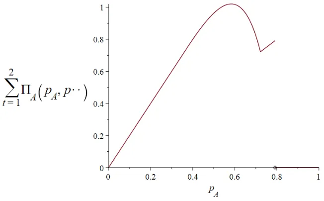
Figure 1: The curve shows A’s payo¤ function for pB =p = 7=12 = 0:583, conditional on the

equilibrium ( ; ) of the BS.

(ii) For any pB 2(0; 1),10 with ( h; k) = ( ; ) A’s payo¤ is

2 X

t=1

E A;t(pA; pB) =

8 > > < > > :

2pA if 0 pA< 3pB₂ 1

pA(EyA)₍e_e;ee)+pA if max 0; 3pB 1

2 pA

1+2pB

3 ;

pA if 1+2₃pB < pA< 1+₂pB

0 if pA 1+₂pB;

(11)

a continuous function of pA for pA 2 0;1+₂pB . Over the range max 0;3pB₂ 1 ;1+2₃pB , @P2t=1E A;t(pA;)

@pA = (EyA)( ; )+pA

d(EyA)₍ ; )

d

@ee

@pA+1, which is positive on a right neighbourhood

of max 0;3pB 1

2 and negative on a left neighbourhood of 1+2pB

3 , while @2P2

t=1E A;t(pA;)

@p2

A < 0:11 _{thus, in that range,}P2

t=1E A;t(pA; )has a unique, internal maximum. P2t=1E A;t(pA; )

is kinked at pA = 1+2₃pB 12 and increasing for pA 2 1+2₃pB;1+₂pB . At a symmetric

equilib-rium, (pA; pB) = (p ; p ) (p = 7=12). (In fact, p = arg max 2 P

t=1

E A;t(pA; p ) since,

while @

2 P

t=1

E A;t(pA; p )=@pA >0 for pA 2 1+2₃p ;1+₂p , P2t=1E A;t(p ; p ) = 49=48>

lim_p A!1+₂p

2 P

t=1

E A;t(pA; p ) = 1+₂p = 38=48 (see Figure 1).

To see why CL raises the …rm’s market power, note that

@

2

P

t=1

E A;t(pA;pB)

@pA j(pA;pB)=(p;p)reads

10_{One can easily prove that, with(}

h; k) = ( ; ),pi= 1(as well aspi= 0) is never a best response. 11@2P2t=1E A;t(pA;)

@p2

A = 2

d(EyA)( ; )

d

@ee

@pA + pA

d2(EyA)( ; )

d 2 @

e e

@pA 2

+ pA

d(EyA)( ; )

d

@2ee

@p2

A, with

@ee

@pA = 5(1 pB)

(2 pA pB)2 <0and

@2_e

e

@p2 A =

10(1 pB) (2 pA pB)3 <0.

12_lim pA!(

1+2pB 3 )

@P2t=1E A( )

@pA =

1 17pB

5(1 pB) <0<limpA!(

1+2pB 3 )

+@

P2

t=1E A( )

2 (EyA)_(1=2;1=2)+ 2p

d(EyA)( ; )

d j =1₂ @p@eA j(pA;pB)=(p;p)= 2

3

4 + (

3 2

p

1 p) under equilibrium

( ; ) and (EyA)_(1=2;1=2) + 1 +p

d(EyA)( ; )

d j =1

2

@ee

@pA j(pA;pB)=(p;p)=

3

4 + 1 + ( 5 4

p 1 p)

under equilibrium ( ; ). Now, 3₄ + 1 > 2 3₄ and 5₄₁p_p > 3₂₁p_p: either inequality follows since ( ; ) implies full capacity utilization in t = 2. Thus, the incentive to unilaterally increasing pA is higher under equilibrium ( ; ) and, as a consequence,

@

2

P

t=1

E A;t(pA;pB)

@pA >0at (pA; pB) = (p ; p ).

4

Conclusion

Our duopolistic price game with a two-buyer dynamic BS provides two main insights. First, even with product homogeneity, repeat purchasing decisions over the time period in which prices are …xed creates an incentive for conditional loyalty. Quite remarkably, this incen-tive arises even with no service priority to loyal customers and with imperfect information on other buyers’ previous moves. Second, the equilibrium of the BS exhibiting conditional loyalty does a¤ect the …rm’s market power. Whether similar results arise in more general models is an issue that we leave to future research. One might check whether a (properly de-…ned) strategy incorporating conditional loyalty is again part of an "assessment equilibrium" of the BS whenn buyers are playing a multistage BS in the face of m sellers;13 _furthermore,

one might explore how such an equilibrium would a¤ect pricing as well as entry and capacity decisions.

References

[1] Binmore, K. (1992) Fun and Games, D. C. Heath: Lexington, Mass.

[2] Burdett, K., Shi, S., and Wright, R. (2001) Pricing and matching with frictions,Journal of Political Economy, 109(5), 1060-1085.

[3] De Francesco, M. A. (1998) The emergence of customer markets in a dynamic buyer game, Quaderni del Dipartimento di Economia Politica, Working Paper 225. Siena.

[4] De Francesco, M. A. (2005) Matching buyers and sellers, Economics Bulletin, 3(31), 1-10.

[5] Deneckere, R., and Peck, J. (1995) Competition over price and service rate when demand is stochastic: a strategic analysis, Rand Journal of Economics, 26(1), 148-162.

[6] Geromichalos, A. (2014) Directed search and the Bertrand paradox,International Eco-nomic Review,55(4), 1043-1065.

13_{Under equal prices at the competiting …rms, partial results in a game theoretic framework are in De}

[7] Goldman, C. V., Kraus, S., and Shehory, O. (2004) On experimental equilibria strategies for selecting sellers and satisfying buyers, Decision Support Systems,38(3), 329-346.

[8] Kreps, D. M., and Wilson, R. (1982) Sequential equilibria, Econometrica, 50(4), 863-894.

[9] Peters, M. (1984) Bertrand equilibrium with capacity constraints and restricted mobil-ity, Econometrica,52(5), 1117-1128.

[10] Shi, S. (2016), Customer relationship and sales, Journal of Economic Theory, 166(C), 483-516.

APPENDIX

Proof of Prop. 3. In BSs where system (9) holds, Uh( ; ) = 2 X

t=1

uh;t( ; ),

where

uh;1( ; ) = ee 2

2 +ee(1 ee)

!

(1 pA) +

(1 ee)2

2 + (1 ee)ee

!

(1 pB); (12)

and14

uh;2( ; ) = X

eh;12Eh;1

(eh;1)₍

h;1; k;1)uh;2( ; j(eh;1; )) =

(Ash;1)₍

h;1; k;1)uh;2( ; j(Ash;1; ))+

(Arh;1)₍

h;1; k;1)uh;2( ; j(Arh;1; ))+

(Bsh;1)₍

h;1; k;1)uh;2( ; j(Bsh;1; ))+

(Brh;1)( _h;1; _k;1)uh;2( ; j(Brh;1; )) = ee2

2 +ee(1 ee)

!

[1 pA] +ee 2

2 [1 pB]+ (1 ee)2

2 + (1 ee)ee

!

[1 pB] +

(1 ee)2

2 [1 pA]: (13)

If h involves a deviation only in t = 1 (i.e., h;1 6= ee), Uh( h; ) = Uh( ; )

(see Remark 3). If h involves a deviation only in t = 2, some of the following hold: 14_{For instance, in Eq. (13), (As}

h;1)₍

h;1; k;1)=

e e2

2 +ee(1 ee) sinceAsh;1= (Ash;1\Ark;1)[(Ash;1\

Bsk;1); also,uh;2( ; j(Ash;1; )) = 1 pA is buyerh’s stage-2 payo¤, under strategy pro…le( ),

h;2(Ash;1; )<1, h;2(Arh;1; )>0; h;2(Bsh;1; )>0, h;2(Brh;1; )<1. Then:

uh;2( h; ) =

X

eh;12Eh;1

(eh;1)₍

h;1; k;1)uh;2( h; j(eh;1; )) =

ee2

2 +ee(1 ee)

!

h;2(Ash;1; )(1 pA) + (1 h;2(Ash;1; ))

1 pB

2 + (14)

ee2

2 h;2(Arh;1; )

1 pA

2 + (1 h;2(Arh;1; ))(1 pB) + (1 ee)2

2 + (1 ee)ee

!

h;2(Bsh;1; )

1 pA

2 + (1 h;2(Bsh;1; ))(1 pB) + (1 ee)2

2 h;2(Brh;1; )(1 pA) + (1 h;2(Brh;1; ))

1 pB

2 ; (15)

Since system (9) holds, system (20_{) a fortiori holds (see Remark 1). As a consequence,}

uh;2( h; j(eh;1; ))< uh;2( ; j(eh;1; ))at any (eh;1; ) where h deviates from .

Let, for instance, h;2(Ash;1; )<1. Then uh;2( h; j(Ash;1; )) = h;2(Ash;1; )(1 pA) +

(1 h;2(Ash;1; ))1 ₂pB < uh;2( ; j(Ash;1; )) = 1 pA, since pA< 1+₂pB.

Next, let system (20_{), but not system (9), hold:}15 _{for instance,} 1+2pB

3 < pA < 1+pB

2 , so

that prescribes _h;1 = 0 and CL. The argument remains essentially unaltered if h

en-tails a one-stage deviation int= 2. With a one-stage deviation int= 1,

2 X

t=1

uh;t( h; ) =

h;1(1 pA) + (1 h;1)1 ₂pB + h;1(1 pA) + (1 h;1) 1₂(1 pB) + 1₂(1 pA , less than 2

X

t=1

uh;t( ; ) = 1 ₂pB + 1₂(1 pB) + 1₂(1 pA) since 1+2₃pB < pA.

Finally, one can easily check that a two-stage deviation from is not rewarding (the "one-stage deviation property" holds).