Modelling crude oil-petroleum products’
price nexus using dynamic conditional
correlation GARCH models
Yaya, OlaOluwa and Ogbonna, Ahamuefula
31 December 2018
Online at
https://mpra.ub.uni-muenchen.de/91227/
Abstract - Modelling volatility in returns has continued to gain popularity with the evolution of the GARCH-type models
under different frameworks. This study therefore examined the different variants of the multivariate GARCH model with focus on those that incorporated asymmetry and constant or dynamic conditional correlations. These variants were used in modelling the crude oil-petroleum products’ (gasoline, heating oil, kerosene, propane and diesel) price nexuses. Comparatively, the DCC-VAR-AMGARCH model fitted the return series more appropriately in four out of the five investigated nexuses, while the DCC-AMGARCH variant fitted the return series in just one nexus. With the exception of propane own market spillover, the overall volatility persistence of spillovers from own market and other markets for the nexuses of crude oil and the other four petroleum products (gasoline, heating oil, diesel and kerosene) were mean reverting. The study also adopted two hedging strategies, for each of the five crude oil-petroleum product nexuses, to ascertain plausible portfolio investment options. The empirical evidence on the different portfolio investments that were herein provided are especially useful for stakeholders/investors desiring to channel their resources into less risky investment portfolios.
Keywords: Asymmetry, Hedging Strategy, Multivariate, Portfolio Management, West Texas Intermediate
1. INTRODUCTION
The drastic drop in global oil prices experienced between 2014 and 2017 was as a result of the excess supply of oil and the ensuing competition in the oil market, which was induced by the shale revolution [1], [2]. In addition, the levels of economic, political crisis and/or stability in oil producing economies contribute immensely to the pricing of oil as it affects supply and consequently, affects the prices of distilled petroleum products such as, gasoline, diesel, kerosene, heating oil and propane. This in a way determined the availability (shortage and/or scarcity, or excess and/or surplus) and quantity of oil supplied in the market, such that a slight or abrupt disruption influences the oil price. In other words, supply shocks, which are transmitted in form of volatility, often affect the pricing of oil, consequently affects consumers, marketers, producers, as well as economic policy makers. Consequent upon the foregoing, there is a growing interest among researchers in the oil market related research. This is, however, not unexpected given the International Energy Agency (IEA) projection that oil will provide up to 30% of the world energy mix by 2030 [3].
Making adequate policy decisions, as well as, setting up appropriate hedging strategies for oil price and its constituent products have been enhanced recently, given the developments of prominent volatility models and modelling studies in extant literature. The Generalized Autoregressive Conditional Heteroscedasticity (GARCH) framework is one prominent developed model that comes in handy in this regard. The model, originally designed in its univariate form for only one variable, was expanded by [4] to the multivariate form - the Multivariate GARCH (MGARCH) model, which can be used to determine
+Economic and Financial Statistics Unit,
Department of Statistics, University of Ibadan, Nigeria.
*Centre for Econometric and Allied Research (CEAR), University of Ibadan, Nigeria
market spillovers. Subsequently, other extensions such as the Constant Conditional Correlation [hereafter, CCC] model of [5] and Dynamic Conditional Correlation [hereafter, DCC] model of [6], which allowed the researcher to obtain the constant and dynamic correlations, respectively, between two conditional variance series from the two variables under investigation, were developed. The CCC and DCC models allowed for conditional correlations and returns spillovers, but do not allow for shock spillovers/interdependencies across markets. As a result of this limitation, [7] proposed a Vector Autoregressive-MGARCH (VAR-Autoregressive-MGARCH) model to accommodate interdependencies of both returns and shocks across financial markets. VAR-MGARCH model is flexible in the sense that it also allows for both constant and dynamic correlations, as in the cases of CCC and DCC models, respectively. The asymmetric version of VAR-MGARCH is given in [8], which includes the leverage parameter in the MGARCH specification of the model. These informed the consideration of the symmetric and asymmetric version of the VAR-MGARCH model that were examined in this study.
In another research, [9] investigated the asymmetric response of gasoline price to crude oil price and found gasoline price to respond more quickly to increases in crude oil price than to decreases, thereby empirically validating the importance of capturing the inherent asymmetric characteristics of oil price series when modelling Crude Oil-Gasoline nexus. In the analysis of future prices of energy commodities such as crude oil, heating oil, gasoline and natural gas, with agricultural commodities such as corn, oats meal, soybean and wheat using the DCC multivariate GARCH models, [10] found significant returns spillovers and conditional correlations
1
Corresponding author;
Tel: + 234 (0) 802 885 6320, +234 (0) 816 787 5650
E-mail: [email protected], [email protected]
Modelling Crude Oil-Petroleum Products’ Price Nexus Using Dynamic Conditional Correlation GARCH Models
among energy and agricultural prices. There has also been research on the volatility spillovers with respect to the exchange rate market and major petroleum products’ market. Specifically, [11] investigated the asymmetric volatility spillovers and portfolio diversification strategy between US dollar-Euro exchange rate market and major petroleum products market such as WTI oil, Brent oil, kerosene, gasoline and propane using bivariate exponential GARCH (EGARCH) model in a DCC framework. Their results indicated significant asymmetric volatility spillovers between the exchange rate and the considered petroleum product markets. Also, their results further showed that structural breaks play dominant role in the modelling of the nexus between any two asset markets. Olubusoye and Yaya [2] investigated jumps and asymmetry in volatility of crude oil and its distilled petroleum products using the univariate framework. The observed persistence of volatility for crude oil and gasoline was lesser compared to the persistence of volatility of crude oil and other petroleum products. Furthermore, jump volatility models with asymmetry and APARCH model proved to predict conditional variances of returns of these prices better than non-jump robust GARCH variants.
In this paper, attempt is made to contribute to the literature in two main ways. First, in a comparative manner, the different extant multivariate models and model combinations (incorporating asymmetry and constant or dynamic conditional correlations) that are usually adopted for capturing returns and volatility spillovers are examined. While adopting these contending models, separately, to model the returns and volatility spillovers from crude oil prices to petroleum products (gasoline, diesel, kerosene, heating oil and propane) prices, the performance of the models are examine when the price series are characterized by some salient statistical features. The aim here is to ascertain the most preferred GARCH-based model variant for each oil-petroleum product nexus, under different scenarios that were structured by incorporating CCC and DCC frameworks into the model, while separately neglecting and/or accounting for inherent asymmetric nature of prices. Secondly, following from the first goal of this study, the oil-petroleum product portfolio investments are examined under two different risk minimization strategies, which provide useful information and guidance on adequate portfolio management and hedging options for policy makers and oil market stakeholders. This is in a view to provide evidence-based alternatives or safe havens for crude oil-petroleum products’ portfolio holders. Following from the introductory part, section 2 provides brief description of the materials and methods employed in the study, with focus on the variant of the GARCH-based model. In section 3, the analysis results are presented and discussed adequately, with necessary implications for stakeholders, while the paper is then concluded in the fourth section.
2. MATERIALS AND METHODS
Time series data used in this paper are the weekly spot prices of crude oil and its petroleum products. These are prices for: Cushing West Texas Intermediate (WTI) oil, Coast conventional regular gasoline, New York Harbor
heating oil, Los Angeles Ultra low sulphur diesel, US Golf Coast kerosene-type Jet fuel and Mont Belvieu propane. The start and end dates for each of the series in this study are 19 April 1996 and 4 May 2018, respectively. The dataset was retrieved from the database in the website (http://www.eia.gov/dnav/pet/pet_pri_spt_s1_w.htm) of the United States Energy Information Administrations (EIA). Crude oil is sold at the market in US dollar/barrel, while the constituent petroleum products are sold in US dollar/gallon.
Subsequently, the continuous compounded log-returns of the prices of the time variables were obtained using equation 1, as given below,
1
ln
1
i i i
t t t
R
P P
where
R
ti was used to represent the log-returns of the given petroleum price series at time t,P
ti was used to represent the price of petroleum product at time t, while1
i t
P
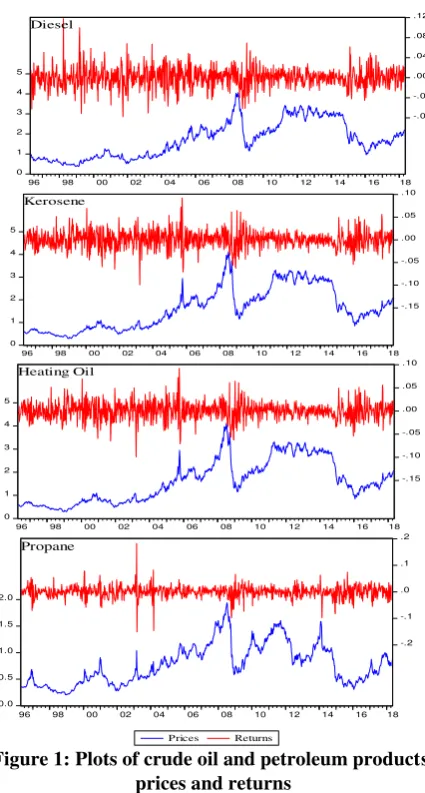
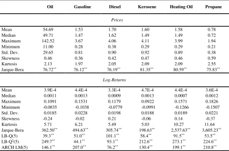
represented the one time period lag of the petroleum product price of interest. Having generated the return series, the historic pattern and statistical distributions of the all considered prices and their corresponding return series were examined using some descriptive statistics.First, though informally and subjectively, the historic behaviour of these prices and their corresponding returns were displayed graphically in Figure 1 below. A quick examination of the six plots revealed similar patterns in the six prices considered, which could be indicative of plausible movement among the prices. The co-movements in the price series, while generally upward trending, were observed to have been greatly influenced by two prominent global events – the global financial crisis of 2007/2008 and the oil price crash of 2014/2015. These events caused prices to drop drastically. On the returns, volatility clustering, as well as price jumps, were highly pronounced in the plots. The preliminary data analyses on the prices and log-returns of the petroleum products revealed the inherent statistical properties of the series being examined and also confirmed the presence of volatility in the return series (see the results in Table 1). The upper and lower panels of Table 1 presents the results for crude oil and petroleum products’ prices and return series, respectively.
0 40 80 120 160
-.10 -.05 .00 .05 .10 .15
96 98 00 02 04 06 08 10 12 14 16 18
Crude Oil
0 1 2 3 4
-.12 -.08 -.04 .00 .04 .08 .12 .16
96 98 00 02 04 06 08 10 12 14 16 18
3
0 1 2 3 4 5 -.08 -.04 .00 .04 .08 .12
96 98 00 02 04 06 08 10 12 14 16 18
Diesel
0 1 2 3 4 5 -.15 -.10 -.05 .00 .05 .10
96 98 00 02 04 06 08 10 12 14 16 18
Kerosene
0 1 2 3 4 5 -.15 -.10 -.05 .00 .05 .10
96 98 00 02 04 06 08 10 12 14 16 18
Heating Oil
0.0 0.5 1.0 1.5 2.0 -.2 -.1 .0 .1 .2
96 98 00 02 04 06 08 10 12 14 16 18
Prices Returns
Propane
Figure 1: Plots of crude oil and petroleum products’ prices and returns
The mean crude oil price was 54.7 USD/barrel, while the respective average prices for gasoline, diesel, kerosene, heating oil and propane laid in the range of 1.5 – 1.60 USD/gallon. Crude oil price rose as high as 142.5 USD/barrel, while it recorded a historic low of 11.0 USD/barrel as indicated by the minimum. The period corresponding to this historic low global selling price of crude oil (WTI) marks the period when crude oil sales was not lucrative. The standard deviation values were very high, almost half of the mean price in each case, showing high data variations in the series, which was suggestive of the price series being highly volatile. Furthermore, the prices were positively skewed, low peaked and thin tailed (platykurtic). Since volatility were observed in the log-return series of prices, similar descriptive measurements and pre-tests for the return series were also obtained (see
the lower panel of Table 1). On the average, the mean returns for crude oil was 0.00039, with corresponding standard deviation of 0.01850, which further confirmed the high volatility presence in returns. The return series were negatively skewed in the case of crude oil, gasoline, kerosene and propane, but positively skewed in the case of diesel and heating oil. All the return series were leptokurtic and non-normal, following from the kurtosis statistic and Jarque-Bera normality tests, respectively. The Ljung-Box (LB-Q and LB-Q2) and the ARCH LM test statistics, all
tested at lag 5, were found to be statistically significant at 5% level, which is indicative of the presence of serial
[image:4.595.82.295.47.444.2]correlation and heteroscedasticity in the return series. Consequently, the presence of ARCH effect informed the appropriateness of the GARCH-based model adopted in this study.
Table 1: Descriptive statistics (oil and petroleum product prices and returns)
Intentionally Left Blank
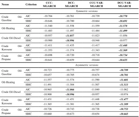
Next, the models to be adopted in the study were extensively specified by including different model combinations, based on the choice to either account for asymmetry or not to, and assuming either constant or dynamic conditional correlations. The resulting GARCH-based models were used to model the nexuses and subsequently compared, one to the others. Using the popular model selection criteria (usually employed when researchers were confronted with selecting a preferred model from a list of several plausible contending goods models) - Akaike information criterion (AIC) and Swartz-Bayesian information criterion (SBIC), the preferred model(s) that best fitted the price and return series were selected (see the results in Table 2).
Table 2: Model specification result
Intentionally Left Blank
The selection was based on the model with the least information criterion measure. Generally, the contending GARCH model (MGARCH and VAR-MGARCH) variants that incorporated dynamic conditional correlation were observed to have the least loss of information in comparison with the GARCH model variants that incorporated constant conditional correlation. This stance was observed across the five crude oil-petroleum products’ nexuses, which informed the consideration of the GARCH model with dynamic conditional correlation incorporated under both the symmetric and asymmetric versions. For crude oil-gasoline, crude oil-heating oil, crude oil-kerosene and crude oil-propane nexuses, the DCC-VAR-MGARCH model and its asymmetric version (DCC-VAR-AMGARCH) were favoured by the employed data under the symmetric and asymmetric versions, respectively, while for crude oil-diesel nexus, the preferences were the DCC-MGARCH and DCC-AMGARCH models under the symmetric and asymmetric versions, respectively (see Table 2). However, in choosing between the symmetric and asymmetric versions of the preferred GARCH models in each nexus, as a way of determining the importance of asymmetries, the latter version seemed to outperform the former. This consequently suggested that in capturing the crude oil-petroleum products’ nexuses, one must account for the presence of asymmetries. Also, incorporating the DCC, rather than the CCC, may further improve upon the parameter estimates in each nexus.
The VAR-MGARCH model with dynamic conditional correlation (DCC-VAR-MGARCH) was specified with the conditional mean equation, conditional probability distribution and conditional variance equation. The conditional mean equation was given in equation 2:
0 1 1
2
t t t
where
R
t
r
tOr
tP
withr
tO andr
tP being the returns on the crude oil market price and petroleum products’ market prices, respectively, at time t;
1 is a
2 2
matrix of coefficients of the form1 1 1 1 1 OO OP PO PP
;
0 is a
2 1
vector of constantsterms of the form
0O
0P
;
t
tO
tP
with Ot
and
tP being the error terms from the mean equations of the crude oil market and petroleum products market returns, respectively.The conditional probability distribution for the GARCH error is as specified in equation 3 below;
3
t
D z
t t
where
z
tz
tOz
tP
referred to a
2 1
vector of independently and identically distributed errors, and
O P
t t t
D
diag
h
h
withh
tO andh
tPrepresenting the conditional variances of crude oil returns
O tr
and petroleum products’ returns
r
tP , respectively, from respective univariate GARCH variants. In this study, the GJR-GARCH model, an asymmetric model type, was considered in conformance to the earlier detected salient feature of the price and return series in the preliminary analyses (see Table 3). The GJR-GARCH model was a prominent GARCH extension developed by [12] et al. (1993), which incorporated an asymmetric term to capture the leverage effect (that is, the effect of negative shock in equity prices on volatility).The conditional variance equation in equation 4 below is of the form,
1 1 1 1
4
i
t t t t t t
H A
A C I z
CB H Bwhere A and B are square matrices, and C and
are diagonal matrices, defined as,1 1 1 1 OO OP PO PP
a
a
A
a
a
, 1 1 1 1 OO OP PO PPb
b
B
b
b
, 1 10
0
OO PPc
C
c
, and0
0
OO PP
.From equation 4 above,
H
t represented the conditional variance-covariance matrix, with the elements of the matrix A being the ARCH coefficients. This showed the effect of past shock in the own market and shock spillovers from the other market, on the current conditional volatility of the other market. Also, elements of matrix Bare the GARCH coefficients that showed the effects of past volatilities in own market and past volatility spillovers from the other market, on the current conditional volatility. The ARCH terms indicated short term persistence of volatility, since the effect of shock in the conditional
volatility was not expected to last long, while GARCH terms indicated long term persistence of volatility. The sum of the ARCH and the GARCH terms, for a particular market, indicated the overall volatility persistence. This sum was expected to be less than unity, which consequently implied the plausibility of mean reversion in volatility. Mean reversion, in this sense, implied the possibility of temporal effect of volatility transmission between two asset prices at the market. Sums that were equal to or greater than unity indicated non-mean reversion, that is, volatility effects will last long, possibly requiring strong intervention from policy makers.
The elements of matrix C represented asymmetric effects, showing significance of asymmetric effects for own markets. The significance of asymmetric effect in a market implied that negative shock (bad news) imparted higher conditional volatility than positive shock (good news). This effect was captured by the conditional indicator,
ti
i t
0,
0
5
1,
0
i t
I z
where
i
indicated the selected market at time t.For the constant conditional correlation (CCC) specification in the asymmetric VARMA-MGARCH (VARMA-AMGARCH) framework, let
H
t1 2
D
t then,
1 1
6
t t t
D H D
where
D
t
diag
h
tOh
tP
, and
OP was the constant conditional correlation between the conditional variances of the two asset price returns.For the conditional variance in the case of the asymmetric DCC-VARMA-MGARCH (DCC-VARMA-AMGARCH) model, the dynamic conditional correlation matrix was obtained by computing,
1 2
1 2
7
t t t
diag H
H diag H
and
H
t was a positive definite matrix given as,
1 2 1 1 1 1 2 11
8
t t t t t
H
H
I
H
where
1 and
2 were non-negative parameters, measuring the effects of previous shocks and previous conditional volatility on the current conditional volatility. Thus, by imposing the restriction,
1
2
0
,t
H
H
, such that the DCC-VARMA-GARCH model reduced to CCC-VARMA-GARCH model.5
2.1 PORTFOLIO MANAGEMENT AND HEDGING
STRATEGY
The significance of returns and volatility spillovers between two markets implied that investors’ assets in the markets were volatile and prone to risk. Thus, to avoid such risk, trade participants need to adopt appropriate hedging strategies. Two hedging strategies were thus determined in this paper, which included: optimal portfolio weight and optimal hedge ratio. Both served as benchmarks for risk minimization strategies in portfolio investments.
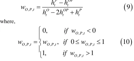
The optimal portfolio weight determined the optimal amount of each asset to be included in the investment portfolio. Following [15], the optimal weight of holding crude oil (O) and petroleum products (P) was given in equation 9 as,
, ,
9
2
P OP
t t
O P t O OP P
t t t
h
h
w
h
h
h
where,
, ,, , , , , , , ,
0,
0
, 0
1
10
1,
1
O P t
O P t O P t O P t
O P t
if w
w
w
if
w
if w
where
w
O P t, , represented the weight of crude oil in one-dollar of crude oil-petroleum product portfolio at a given time t,h
tOandh
tPwere the conditional variances of oil andpetroleum products, respectively,
h
tOP represented the conditional covariance between crude oil and petroleum product returns at time t, and the optimal weight of petroleum product in one-dollar of the portfolio of the two assets was obtained using1
w
O P t, , .As another risk minimization strategy, [16] provided an optimal (minimum variance) hedge ratio, with the believe that the risk of the investment portfolio was minimized, if a long position of one dollar in the crude oil market was hedged by a short position of
t dollars in the petroleum product market. The optimal hedge ratio
O P t, ,
between the two assets (crude oil and selectedpetroleum product) was given in equation 11 as,
, ,
11
OP t
O P t P
t
h
h
where
h
tOPandh
tP remained as previously defined. This minimization strategy gave a quantifiable measure of the risk that a portfolio holder was exposed to given his choice of portfolio to invest in.3. RESULTS AND DISCUSSION
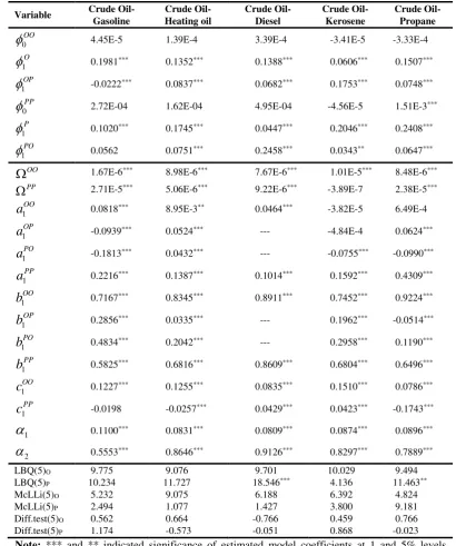
Table 3 showed the results of the AMGARCH variance models for VARMA, and DCC mean specifications for petroleum product price returns, as detected by minimum information criteria in Table 2. The results were divided into three segments: the first presented the estimates of the parameters of the mean equation; the second presented the
estimates of the parameters of the variance equation, while the last segment presented some relevant diagnostic test results on the overall model residuals.
[image:6.595.72.307.245.352.2]Looking at the mean equation results presented in the first segment of Table 3, the estimates of the autoregressive parameters
1O and
1P, for both crude oil price returns and petroleum product price returns, respectively, were statistically significant, even at 1% levels. These implied the dependences of current returns of crude oil and petroleum products on their respective immediate past returns. These also justified the allowance of theARMA
1,1
specification, instead of the pure AMGARCH specification for those nexuses. There were statistically significant returns’ spillovers from petroleum products’ price returns to crude oil price returns
1OP for the five nexuses, while in the cases of petroleum products and crude oil price returns nexuses
1PO , except for Crude Oil-Gasoline nexus that indicated no significant cross spillover, the remaining four nexuses showed significant crude oil-petroleum products’ price returns spillovers. The fact that there was no significant spillover from crude oil price to gasoline price justified the fact that gasoline demand was the highest among the considered petroleum products.Table 3: Estimated models
Intentionally Left Blank
own markets except propane own market in the crude oil-propane nexus. The asymmetric parameters
c
1OO andc
1PPwere also significant, justifying the applicability of AMGARCH specification for the variance component of the models. These further confirmed the outperformance of the asymmetric version over the symmetric version given by the information criteria (see results in Table 2). For the dynamic correlation structure, Crude Oil-Gasoline nexus indicated the lowest persistence of dynamic correlation 0.6653 (sum of
1 and
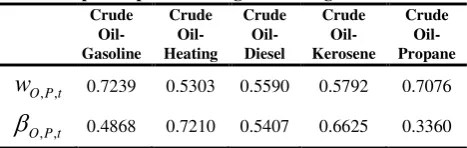
2), while the highest was observed in the case of crude oil-heating oil nexus (0.9935). By looking at the diagnostic tests in the last segment, the results based on Ljung-Box and McLeod-Li statistics indicated adequacy of the estimated models for all the considered nexuses. The Difference test statistic (Diff.test) investigated for the presence of asymmetry in the residuals of each model, and in each case, there was no remaining asymmetry in the residuals of the preferred models for the different nexuses. [image:7.595.36.270.609.683.2]Table 4 displayed the optimal portfolio weights and the optimal hedge ratio for each pair of crude oil-petroleum product nexus. In the case of crude oil-gasoline nexus, the average weight of holding crude oil in a one-dollar crude oil-gasoline portfolio was 72.4%, while the balance of 27.6% was to be invested in gasoline market. For crude oil-heating oil, crude oil-diesel and crude oil-kerosene portfolios, the average weights of crude oil in a one-dollar portfolio for each of the nexus was 53.0%, 55.9% and 57.9%, respectively, with the balance of 47.0%, 44.1% and 42.1% to be invested in heating oil, diesel and kerosene markets, respectively. In the case of crude oil-propane nexus, 70.8% of oil was expected to be invested in one-dollar crude oil-propane portfolio, while the balance of 29.2% should be invested in propane. The overall result indicated that investors in crude oil and its petroleum products were likely to be worst off by holding more of crude oil than gasoline and propane in the crude oil-gasoline and crude oil-propane portfolios, respectively, whereas in the case of heating oil, diesel and kerosene, the demand was slightly higher for crude oil than these petroleum products (heating oil, diesel and kerosene), and this may serve as incentive for investing in crude oil, instead of its distilled petroleum products.
Table 4: Optimal portfolio weight and hedge ratio
Crude Oil-Gasoline
Crude Oil-Heating
Crude Oil-Diesel
Crude Oil-Kerosene
Crude Oil-Propane
, ,
O P t
w
0.7239 0.5303 0.5590 0.5792 0.7076, ,
O P t
0.4868 0.7210 0.5407 0.6625 0.3360Source: Computed by the authors
On the optimal hedge ratio, and in the case of crude oil-gasoline and crude oil-propane portfolios, one dollar long in crude oil should be shorted by 48.7% and 33.6% of gasoline and propane, respectively. However, for crude oil-heating oil, crude oil-diesel and crude oil-kerosene, a long position of one dollar investment in crude oil market is taken, that is, crude oil was shorted by 72.1%, 54.1% and 66.5%, respectively, of heating oil, diesel and kerosene.
4. CONCLUDING REMARKS
This study set out to model crude oil-petroleum products’ price nexus using several variants of the GARCH model. More specifically, the study attempted to accomplish two major goals. Firstly, to examine the appropriateness of different specifications of the GARCH type model (including model combinations that incorporate asymmetry and constant or dynamic conditional correlations) for capturing returns and volatility spillovers from crude oil (WTI) price (in USD/barrel) to petroleum products (gasoline, diesel, kerosene, heating oil and propane) prices (in USD/gallon). Secondly, to examine two risk minimization strategies, with the view to recommend appropriate hedging options in the five pairs of crude oil-petroleum products’ portfolios, which could be useful to policy makers, and crude oil and its distilled constituents’ market stakeholders.
Following from the preliminary analyses, which confirmed the non-normality characteristics of all the series considered, asymmetric nature of crude oil price return series were further confirmed with evidence of weak asymmetry in the case of diesel price return series. DCC tests for the five nexuses investigated were also found to be significant. These informed the adoption of the
asymmetric MGARCH (AMGARCH) and the
incorporation of dynamic conditional correlations, to capture the bivariate crude oil-petroleum products nexus, hence the adopted specification - DCC-VAR-MGARCH. On the comparative assessment of the different variants of the conventional GARCH models, DCC-VAR-AMGARCH model was found to be favoured by the data used in the crude oil-gasoline, crude oil-heating oil, crude oil-kerosene and crude oil-propane nexuses, while the crude oil-diesel nexus was best captured using DCC-AMGARCH model. In all the nexuses, the overall volatility persistence was mean reverting, both for spillovers from other markets and spillovers from own market except propane in the crude oil-propane nexus. Thus, the crude oil-propane modelling may require some level of interventions.
Finally, while adopting two hedging strategies (optimal portfolio weight and optimal hedge ratio), the study showed the optimal proportion of each asset to include in one dollar investment portfolio and the feasible proportion of same to be shorted within any given portfolio. These would enable the trade participants adopt appropriate hedging strategies, while avoiding the inherent unguided risk associated with the market volatility.
REFERENCES
[1] Gil-Alana, L.A., Gupta, R., Olubusoye, O.E. and Yaya, O.S., 2016. Time Series Analysis of Persistence in Crude Oil Price Volatility across Bull and Bear Regimes. Energy, 109: 29-37.
[2] Olubusoye, O.E. and Yaya, O.S., 2016. Time Series Analysis of Volatility in the Petroleum Markets: The Persistence, Asymmetry and Jumps in the Returns Series. OPEC Energy Review, 42(3): 235-262. [3] International Energy Agency (IEA, 2008). World
7
[4] Baba, Y., Engle, R.F., Kraft, D. and Kroner, K.F., 1990. Multivariate simultaneous generalized ARCH.
Mimeo, Department of Economics, University of California, San Diego.
[5] Bollerslev, T., 1990. Modelling the coherence in short-run nominal exchange rates: A multivariate generalized ARCH approach. Review of Economics and Statistics, 72: 498-505.
[6] Engle, R. F., 2002. Dynamic Conditional Correlation: A simple class of multivariate generalized autoregressive conditional heteroscedasticity models.
Journal of Business and Economic Statistics, 20: 339-350.
[7] Ling, S. and McAleer, M., 2003. Asymptotic Theory for a Vector ARMA-GARCH Model. Econometric Theory, 19: 278-308.
[8] McAleer, M., Hoti, S. and Chan, F., 2009. Structure and asymptotic theory for multivariate asymmetric conditional volatility. Economic Review, 28: 422 - 440.
[9] Borenstein, S., Cameron, A.C. and Gilbert, R., 1997. Do Gasoline prices respond asymmetrically to crude oil price changes? The Quarterly Journal of Economics, 112(1): 305-339.
[10] Manera, M., Nicolini, M. and Vignati, I., 2013. Financial speculation in Energy and Agriculture Futures markets: A Multivariate GARCH approach.
The Energy Journal, 34(3): 55-81.
[11] Mensi, W., Hammoudeh, S. and Yoon, S-M., 2014. Structural breaks, dynamic correlations, volatility transmission and hedging strategies for international petroleum prices and US dollar exchange rate.
Economic Research Forum Working paper no. 884. [12] Glosten, L., Jagannathan, R., and Runkle, D., 1993. On
the relation between the expected value and the volatility of the nominal excess return on stocks.
Journal of Finance 48, 1779-1801.
[13] Bollerslev, T., 1986. Generalized Autoregressive Conditional Heteroscedasticity. Journal of Econometrics, 31, 307-327.
[14] Caporin, M. and McAleer, M.J., 2010. Ranking multivariate GARCH models by problem dimension.
Econometric Institute Research Papers EI 2010-34. Erasmus University Rotterdam, Erasmus School of Economics (ESE).
[15] Kroner, K. and Ng, V., 1998. Modelling asymmetric movements of asset prices. Review of Financial Studies, 11: 844-871.
Table 1: Descriptive statistics (oil and petroleum product prices and returns)
Oil Gasoline Diesel Kerosene Heating Oil Propane
Prices
Mean 54.69 1.53 1.70 1.60 1.58 0.78 Median 49.71 1.47 1.62 1.49 1.49 0.72 Maximum 142.52 3.67 4.06 4.11 3.99 1.94 Minimum 11.00 0.28 0.38 0.29 0.29 0.21 Std. Dev. 29.65 0.81 0.90 0.92 0.89 0.38 Skewness 0.46 0.36 0.42 0.47 0.46 0.59 Kurtosis 2.13 1.97 2.05 2.09 2.09 2.55 Jarque-Bera 76.72** 76.12** 76.19** 81.35** 80.59** 75.83**
Log-Returns
Mean 3.9E-4 4.4E-4 3.3E-4 4.7E-4 4.4E-4 3.6E-4 Median 0.0011 0.0013 0.0009 0.0013 0.0007 0.0012 Maximum 0.1091 0.1531 0.1179 0.0922 0.1571 0.1826 Minimum -0.0835 -0.1038 -0.0779 -0.0991 -0.1266 -0.1507 Std. Dev. 0.0185 0.0228 0.0198 0.0188 0.0189 0.0221 Skewness -0.24 -0.02 0.21 -0.06 0.14 -0.37 Kurtosis 5.71 6.21 5.49 5.03 10.27 11.64 Jarque-Bera 362.50** 494.63** 305.74** 198.63** 2,537.63** 3,605.23** LB-Q(5) 39.3** 51.0** 101.1** 58.4** 91.5** 53.5** LB-Q2(5) 249.7** 44.1** 93.1** 212.6** 273.1** 224.6** ARCH LM(5) 146.1** 207.0** 76.2** 130.4** 199.1** 210.8**
Note: ** represents significant of Jarque-Bera, Ljung-Box and ARCH LM tests at 5% level. The Jarque-Bera tests the null hypothesis of series normality against non-normality. The LB-Q(5) and LB-Q2(5) test for standardized
residuals and their squares, respectively, while the ARCH LM indicates the Lagrangian Multiplier test for Autoregressive Conditional Heteroscedasticity. The reported statistic for the ARCH LM is nR2, where n and R2
9
Table 2: Model specification result
Nexus Criterion CCC-MGARCH
DCC-MGARCH
CCC-VAR-MGARCH
DCC-VAR-MGARCH Symmetric versions
Crude Oil-Gasoline
AIC -10.704 -10.761 -10.739 -10.770
SBIC -10.646 -10.700 -10.664 -10.691
Oil-Heating AIC -11.540 -11.558 -11.559
-11.578
SBIC -11.483 -11.497 -11.484 -11.499
Crude Oil-Diesel AIC -10.957
-11.057 -11.023 -11.056
SBIC -10.900 -10.996 -10.948 -10.977
Crude Oil-Kerosene
AIC -11.411 -11.435 -11.417 -11.448
SBIC -11.353 -11.374 -11.343 -11.369
Crude Oil-Propane
AIC -10.698 -10.720 -10.718 -10.734
SBIC -10.641 -10.659 -10.644 -10.655
Asymmetric versions
Crude Oil-Gasoline
AIC -10.723 -10.775 -10.757 -10.789
SBIC -10.657 -10.705 -10.674 -10.701
Oil-Heating AIC -11.557 -11.574 -11.590
-11.601
SBIC -11.491 -11.504 -11.507 -11.513
Crude Oil-Diesel AIC -10.965
-11.066 -11.040 -11.062
SBIC -10.900 -10.996 -10.957 -10.974
Crude Oil-Kerosene
AIC -11.431 -11.451 -11.448 -11.477
SBIC -11.365 -11.381 -11.365 -11.389
Crude Oil-Propane
AIC -10.726 -10.743 -10.738 -10.753
SBIC -10.660 -10.673 -10.654 -10.665
Note: Italicized figures indicate minimum Akaike Information Criterion (AIC) and Swartz Bayesian Information Criterion (SBIC), corresponding to the selected model. The table is divided into two panels, with the first reporting the information criteria for the symmetric versions, while the second reports for the asymmetric version the same model constructs. Bold-Italicized figures in the table indicate the model with the least information criterion among contending models.
Table 3: Estimated models
Variable Crude Oil-Gasoline
Crude Oil-Heating oil
Crude Oil-Diesel
Crude Oil-Kerosene
Crude Oil-Propane
0
OO
4.45E-5 1.39E-4 3.39E-4 -3.41E-5 -3.33E-41
O
0.1981*** 0.1352*** 0.1388*** 0.0606*** 0.1507***1
OP
-0.0222*** 0.0837*** 0.0682*** 0.1753*** 0.0748***0
PP
2.72E-04 1.62E-04 4.95E-04 -4.56E-5 1.51E-3***1
P
0.1020*** 0.1745*** 0.0447*** 0.2046*** 0.2408***1
PO
0.0562 0.0751*** 0.2458*** 0.0343** 0.0647***OO
1.67E-6*** 8.98E-6*** 7.67E-6*** 1.01E-5*** 8.48E-6***PP
2.71E-5*** 5.06E-6*** 9.22E-6*** -3.89E-7 2.38E-5***1
OO
a
0.0818*** 8.95E-3** 0.0464*** -3.82E-5 6.49E-41
OP
a
-0.0939*** 0.0524*** --- -4.84E-4 0.0624***1
PO
a
-0.1813*** 0.0432*** --- -0.0755*** -0.0990***1
PP
a
0.2216*** 0.1387*** 0.1014*** 0.1592*** 0.4309***1
OO
b
0.7167*** 0.8345*** 0.8911*** 0.7452*** 0.9224***1
OP
b
0.2856*** 0.0335*** --- 0.1962*** -0.0514***1
PO
b
0.4834*** 0.2042*** --- 0.2958*** 0.1190***1
PP
b
0.5825*** 0.6816*** 0.8609*** 0.6804*** 0.6496***1
OO
c
0.1227*** 0.1255*** 0.0835*** 0.1510*** 0.0786***1
PP
c
-0.0198 -0.0257*** 0.0429*** 0.0423*** -0.1743***1
0.1100*** 0.0831*** 0.0809*** 0.0874*** 0.0896***2
0.5553*** 0.8646*** 0.9126*** 0.8297*** 0.7889*** LBQ(5)O 9.775 9.076 9.701 10.029 9.494 LBQ(5)P 10.234 11.727 18.546*** 4.136 11.463** McLLi(5)O 5.232 9.075 6.188 6.392 4.824 McLLi(5)P 2.494 1.077 1.427 3.800 9.181 Diff.test(5)O 0.562 0.664 -0.766 0.459 0.766 Diff.test(5)P 1.174 -0.573 -0.051 0.868 -0.023Note: *** and ** indicated significance of estimated model coefficients at 1 and 5% levels, respectively. Model residual diagnostic tests are Ljung-Box Q statistic and McLeod-Li (McLLi) for independence testing of residuals and squared residuals. These are computed for lag 5 of the residuals. Test of Difference Sign (Diff.test) of the residuals are also conducted to investigate the remaining asymmetry in the residuals.