Proceedings of the 55th Annual Meeting of the Association for Computational Linguistics, pages 1535–1546 Vancouver, Canada, July 30 - August 4, 2017. c2017 Association for Computational Linguistics Proceedings of the 55th Annual Meeting of the Association for Computational Linguistics, pages 1535–1546
Vancouver, Canada, July 30 - August 4, 2017. c2017 Association for Computational Linguistics
Lexically Constrained Decoding for Sequence Generation Using Grid
Beam Search
Chris Hokamp
ADAPT Centre Dublin City University
Qun Liu
ADAPT Centre Dublin City University
Abstract
We present Grid Beam Search (GBS), an algorithm which extends beam search to allow the inclusion of pre-specified lex-ical constraints. The algorithm can be used with any model that generates a se-quence ˆy = {y0. . . yT}, by maximizing p(y|x) = Q
t
p(yt|x;{y0. . . yt−1}).
Lex-ical constraints take the form of phrases or words that must be present in the out-put sequence. This is a very general way to incorporate additional knowledge into a model’s output without requiring any modification of the model parameters or training data. We demonstrate the feasibil-ity and flexibilfeasibil-ity of Lexically Constrained Decoding by conducting experiments on Neural Interactive-Predictive Translation, as well as Domain Adaptation for Neural Machine Translation. Experiments show that GBS can provide large improvements in translation quality in interactive scenar-ios, and that, even without any user in-put, GBS can be used to achieve signifi-cant gains in performance in domain adap-tation scenarios.
1 Introduction
The output of many natural language processing models is a sequence of text. Examples include automatic summarization (Rush et al.,2015), ma-chine translation (Koehn, 2010;Bahdanau et al., 2014), caption generation (Xu et al.,2015), and di-alog generation (Serban et al.,2016), among oth-ers.
In some real-world scenarios, additional infor-mation that could inform the search for the opti-mal output sequence may be available at inference
time. Humans can provide corrections after view-ing a system’s initial output, or separate classifi-cation models may be able to predict parts of the output with high confidence. When the domain of the input is known, a domain terminology may be employed to ensure specific phrases are present in a system’s predictions. Our goal in this work is to find a way to force the output of a model to contain suchlexical constraints, while still taking advan-tage of the distribution learned from training data. For Machine Translation (MT) usecases in par-ticular, final translations are often produced by combining automatically translated output with user inputs. Examples include Post-Editing (PE) (Koehn,2009;Specia,2011) and Interactive-Predictive MT (Foster, 2002; Barrachina et al., 2009;Green, 2014). These interactive scenarios can be unified by considering user inputs to be lex-ical constraints which guide the search for the op-timal output sequence.
In this paper, we formalize the notion of lexi-cal constraints, and propose a decoding algorithm which allows the specification of subsequences that are required to be present in a model’s out-put. Individual constraints may be single tokens or multi-word phrases, and any number of constraints may be specified simultaneously.
Although we focus upon interactive applica-tions for MT in our experiments, lexically con-strained decoding is relevant to any scenario where a model is asked to generate a sequence
ˆ
y = {y0. . . yT} given both an input x, and a set {c0...cn}, where each ci is a sub-sequence
{ci0. . . cij}, that must appear somewhere in ˆy. This makes our work applicable to a wide range of text generation scenarios, including image de-scription, dialog generation, abstractive summa-rization, and question answering.
The rest of this paper is organized as follows: Section2gives the necessary background for our
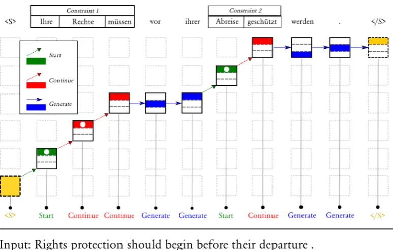
Figure 1: A visualization of the decoding process for an actual example from our English-German MT experiments. The output token at each timestep appears at the top of the figure, with lexical constraints enclosed in boxes. Generationis shown in
blue,Startingnew constraints ingreen, andContinuingconstraints inred. The function used to create the hypothesis at each timestep is written at the bottom. Each box in the grid represents a beam; a colored strip inside a beam represents an individual hypothesis in the beam’sk-best stack. Hypotheses with circles inside them areclosed, all other hypotheses areopen. (Best viewed in colour).
discussion of GBS, Section 3 discusses the lex-ically constrained decoding algorithm in detail, Section4presents our experiments, and Section5 gives an overview of closely related work.
2 Background: Beam Search for Sequence Generation
Under a model parameterized by θ, let the best output sequenceˆygiven inputxbe Eq.1.
ˆ
y= argmax y∈{y[T]}
pθ(y|x), (1)
where we use{y[T]} to denote the set of all se-quences of lengthT. Because the number of pos-sible sequences for such a model is|v|T, where|v| is the number of output symbols, the search foryˆ
can be made more tractable by factorizingpθ(y|x) into Eq.2:
pθ(y|x) = T
Y
t=0
pθ(yt|x;{y0. . . yt−1}). (2)
The standard approach is thus to generate the output sequence from beginning to end, condition-ing the output at each timestep upon the inputx,
and the already-generated symbols {y0. . . yi−t}.
However, greedy selection of the most probable output at each timestep, i.e.:
ˆ
yt= argmax yi∈{v}
p(yi|x;{y0. . . yt−1}), (3)
risks making locally optimal decisions which are actually globally sub-optimal. On the other hand, an exhaustive exploration of the output space would require scoring |v|T sequences, which is intractable for most real-world models. Thus, a search or decoding algorithm is often used as a compromise between these two extremes. A com-mon solution is to use a heuristic search to at-tempt to find the best output efficiently (Pearl, 1984;Koehn, 2010; Rush et al., 2013). The key idea is to discard bad options early, while trying to avoid discarding candidates that may be locally risky, but could eventually result in the best overall output.
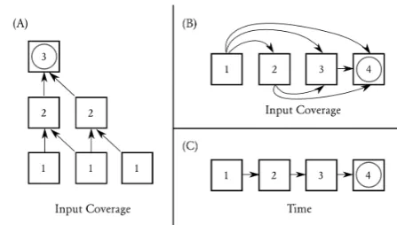
Figure 2: Different structures for beam search. Boxes repre-sent beams which holdk-best lists of hypotheses. (A) Chart Parsing using SCFG rules to cover spans in the input. (B) Source coverage as used in PB-SMT. (C) Sequence timesteps (as used in Neural Sequence Models), GBS is an extension of (C). In (A) and (B), hypotheses are finished once they reach the final beam. In (C), a hypothesis is only complete if it has generated an end-of-sequence (EOS) symbol.
graph of beams can be adapted to take advantage of additional structure that may be available for specific tasks. For example, in Phrase-Based Sta-tistical MT (PB-SMT) (Koehn,2010), beams are organized by the number of source words that are covered by the hypotheses in the beam – a hypoth-esis is “finished” when it has covered all source words. In chart-based decoding algorithms such as CYK, beams are also tied to coverage of the input, but are organized as cells in a chart, which facili-tates search for the optimal latent structure of the output (Chiang, 2007). Figure 2visualizes three common ways to structure search. (A) and (B) de-pend upon explicit structural information between the input and output, (C) only assumes that the output is a sequence where later symbols depend upon earlier ones. Note also that (C) corresponds exactly to the bottom rows of Figures1and3.
With the recent success of neural models for text generation, beam search has become the de-facto choice for decoding optimal output se-quences (Sutskever et al., 2014). However, with neural sequence models, we cannot organize beams by their explicit coverage of the input. A simpler alternative is to organize beams by output timesteps from t0· · ·tN, where N is a hyperpa-rameter that can be set heuristically, for example by multiplying a factor with the length of the in-put to make an educated guess about the maximum length of the output (Sutskever et al.,2014). Out-put sequences are generally considered complete once a special “end-of-sentence”(EOS) token has been generated. Beam size in these models is also typically kept small, and recent work has shown
Figure 3: Visualizing the lexically constrained decoder’s complete search graph. Each rectangle represents a beam containingk hypotheses. Dashed (diagonal) edges indicate startingorcontinuingconstraints. Horizontal edges repre-sentgeneratingfrom the model’s distribution. The horizontal axis covers the timesteps in the output sequence, and the ver-tical axis covers the constraint tokens (one row for each token in each constraint). Beams on the top level of the grid contain hypotheses which cover all constraints.
that the performance of some architectures can ac-tually degrade with larger beam size (Tu et al., 2016).
3 Grid Beam Search
Our goal is to organize decoding in such a way that we can constrain the search space to outputs which contain one or more pre-specified sub-sequences. We thus wish to use a model’s distribution both to “place” lexical constraints correctly, and to gener-ate the parts of the output which are not covered by the constraints.
Algorithm 1 presents the pseudo-code for lex-ically constrained decoding, see Figures 1 and3 for visualizations of the search process. Beams in the grid are indexed by t and c. The t vari-able tracks the timestep of the search, while the c variable indicates how many constraint tokens are covered by the hypotheses in the current beam. Note that each step ofccovers a single constraint token. In other words,constraintsis an array of sequences, where individual tokens can be indexed asconstraintsij, i.e.tokenjinconstrainti. The numCparameter in Algorithm1represents the to-tal number of tokens in all constraints.
The hypotheses in a beam can be separated into two types (see lines 9-11 and 15-19 of Algo-rithm1):
1. openhypotheses can either generate from the model’s distribution, or start available con-straints,
[image:3.595.64.288.60.187.2]Algorithm 1Pseudo-code for Grid Beam Search, note thattandcindices are 0-based
1: procedureCONSTRAINEDSEARCH(model,input,constraints,maxLen,numC,k)
2: startHyp⇐model.getStartHyp(input, constraints)
3: Grid⇐initGrid(maxLen,numC,k) .initialize beams in grid
4: Grid[0][0] =startHyp
5: fort= 1, t++, t < maxLendo
6: forc=max(0,(numC+t)−maxLen), c++, c≤min(t, numC)do 7: n, s, g=∅
8: for eachhyp∈Grid[t−1][c]do
9: ifhyp.isOpen()then
10: g⇐gSmodel.generate(hyp, input, constraints) .generate new open hyps
11: end if
12: end for
13: ifc >0then
14: for eachhyp∈Grid[t−1][c−1]do
15: ifhyp.isOpen()then
16: n⇐nSmodel.start(hyp, input, constraints) .start new constrained hyps
17: else
18: s⇐sSmodel.continue(hyp, input, constraints) .continue unfinished
19: end if
20: end for
21: end if
22: Grid[t][c] = k-argmax
h∈nSsSg
model.score(h) .k-best scoring hypotheses stay on the beam
23: end for
24: end for
25: topLevelHyps⇐Grid[:][numC] .get hyps in top-level beams 26: f inishedHyps⇐hasEOS(topLevelHyps) .finished hyps have generated the EOS token
27: bestHyp⇐ argmax
h∈f inishedHyps
model.score(h)
28: returnbestHyp
29: end procedure
token for in a currently unfinished constraint. At each step of the search the beam at
Grid[t][c]is filled with candidates which may be
created in three ways:
1. the open hypotheses in the beam to the left (Grid[t − 1][c]) may generate
con-tinuations from the model’s distribution pθ(yi|x,{y0. . . yi−1}),
2. theopen hypotheses in the beam to the left and below (Grid[t−1][c−1]) maystartnew
constraints,
3. theclosedhypotheses in the beam to the left and below (Grid[t−1][c−1]) maycontinue
constraints.
Therefore, the model in Algorithm 1
imple-ments an interface with three functions:generate,
start, andcontinue, which build new hypotheses in each of the three ways. Note that the scoring function of the model does not need to be aware of the existence of constraints, but it may be, for ex-ample via a feature which indicates if a hypothesis is part of a constraint or not.
The beams at the top level of the grid (beams where c = numConstraints) contain hypothe-ses which cover all of the constraints. Once a hy-pothesis on the top level generates the EOS token, it can be added to the set of finished hypotheses. The highest scoring hypothesis in the set of fin-ished hypotheses is the best sequence which cov-ers all constraints.1
1Our implementation of GBS is available at https:
3.1 Multi-token Constraints
By distinguishing between open and closed hy-potheses, we can allow for arbitrary multi-token phrases in the search. Thus, the set of constraints for a particular output may include both individ-ual tokens and phrases. Each hypothesis main-tains a coverage vector to ensure that constraints cannot be repeated in a search path – hypotheses which have already coveredconstrainti can only generate, or start constraints that have not yet been covered.
Note also that discontinuous lexical constraints, such as phrasal verbs in English or German, are easy to incorporate into GBS, by addingfiltersto the search, which require that one or more con-ditions must be met before a constraint can be used. For example, adding the phrasal verb “ask hsomeoneiout” as a constraint would mean using “ask” asconstraint0 and “out” as constraint1, with two filters: one requiring that constraint1 cannot be used before constraint0, and another requiring that there must be at least onegenerated token between the constraints.
3.2 Subword Units
Both the computation of the score for a hypoth-esis, and the granularity of the tokens (character, subword, word, etc...) are left to the underlying model. Because our decoder can handle arbitrary constraints, there is a risk that constraints will con-tain tokens that were never observed in the training data, and thus are unknown by the model. Espe-cially in domain adaptation scenarios, some user-specified constraints are very likely to contain un-seen tokens. Subword representations provide an elegant way to circumvent this problem, by break-ing unknown or rare tokens into character n-grams which are part of the model’s vocabulary ( Sen-nrich et al., 2016; Wu et al., 2016). In the ex-periments in Section 4, we use this technique to ensure that no input tokens are unknown, even if a constraint contains words which never appeared in the training data.2
3.3 Efficiency
Because the number of beams is multiplied by the number of constraints, the runtime complexity of a naive implementation of GBS isO(ktc).
Stan-dard time-based beam search isO(kt); therefore, 2If acharacterthat was not observed in training data is observed at prediction time, it will be unknown. However, we did not observe this in any of our experiments.
some consideration must be given to the efficiency of this algorithm. Note that the beams in each col-umncof Figure3 are independent, meaning that GBS can be parallelized to allow all beams at each timestep to be filled simultaneously. Also, we find that the most time is spent computing the states for the hypothesis candidates, so by keeping the beam size small, we can make GBS significantly faster.
3.4 Models
The models used for our experiments are state-of-the-art Neural Machine Translation (NMT) sys-tems using our own implementation of NMT with attention over the source sequence (Bahdanau et al., 2014). We used Blocks and Fuel to im-plement our NMT models (van Merrinboer et al., 2015). To conduct the experiments in the fol-lowing section, we trained baseline translation models for English–German (EN-DE), English– French FR), and English–Portuguese (EN-PT). We created a shared subword representation for each language pair by extracting a vocabulary of 80000 symbols from the concatenated source and target data. See the Appendix for more de-tails on our training data and hyperparameter con-figuration for each language pair. ThebeamSize parameter is set to 10 for all experiments.
Because our experiments use NMT models, we can now be more explicit about the implemen-tations of the generate, start, and continue functions for this GBS instantiation. For an NMT model at timestept,generate(hypt−1)first computes a vector of output probabilities ot = sof tmax(g(yt−1, si, ci))3 using the state infor-mation available fromhypt−1. and returns the best
kcontinuations, i.e. Eq.4:
gt= k-argmax i
oti. (4)
The start and continue functions simply index into the softmax output of the model, selecting specific tokens instead of doing ak-argmax over
the entire target language vocabulary. For exam-ple, tostartconstraintci, we find the score of
to-kenci0, i.e. otci0.
4 Experiments
4.1 Pick-Revise for Interactive Post Editing
Pick-Revise is an interaction cycle for MT Post-Editing proposed byCheng et al.(2016). Starting
ITERATION 0 1 2 3
Strict Constraints
EN-DE 18.44 27.64 (+9.20) 36.66 (+9.01) 43.92(+7.26)
EN-FR 28.07 36.71 (+8.64) 44.84 (+8.13) 45.48+(0.63)
EN-PT* 15.41 23.54 (+8.25) 31.14 (+7.60) 35.89(+4.75)
Relaxed Constraints
EN-DE 18.44 26.43 (+7.98) 34.48 (+8.04) 41.82(+7.34)
EN-FR 28.07 33.8 (+5.72) 40.33 (+6.53) 47.0(+6.67)
[image:6.595.87.514.62.194.2]EN-PT* 15.41 23.22 (+7.80) 33.82 (+10.6) 40.75(+6.93)
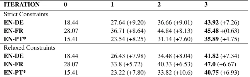
Table 1: Results for four simulated editing cycles using WMT test data. EN-DE usesnewstest2013, EN-FR usesnewstest2014, and EN-PT uses the Autodesk corpus discussed in Section4.2. Improvement in BLEU score over the previous cycle is shown in parentheses. * indicates use of our test corpus created from Autodesk post-editing data.
with the original translation hypothesis, a (sim-ulated) user first picks a part of the hypothesis which is incorrect, and then provides the correct translation for that portion of the output. The user-provided correction is then used as a constraint for the next decoding cycle. The Pick-Revise process can be repeated as many times as necessary, with a new constraint being added at each cycle.
We modify the experiments of Cheng et al. (2016) slightly, and assume that the user only pro-vides sequences of up to three words which are missing from the hypothesis.4 To simulate user interaction, at each iteration we chose a phrase of up to three tokens from the reference transla-tion which does not appear in the current MT hy-potheses. In thestrictsetting, the complete phrase must be missing from the hypothesis. In the re-laxedsetting, only the first word must be missing. Table1shows results for a simulated editing ses-sion with four cycles. When a three-token phrase cannot be found, we backoff to two-token phrases, then to single tokens as constraints. If a hypoth-esis already matches the reference, no constraints are added. By specifying a new constraint of up to three words at each cycle, an increase of over 20 BLEU points is achieved in all language pairs.
4.2 Domain Adaptation via Terminology
The requirement for use of domain-specific termi-nologies is common in real-world applications of MT (Crego et al.,2016). Existing approaches in-corporate placeholder tokens into NMT systems, which requires modifying the pre- and post- pro-cessing of the data, and training the system with
4NMT models do not use explicit alignment between source and target, so we cannot use alignment information to map target phrases to source phrases
data that contains the same placeholders which oc-cur in the test data (Crego et al., 2016). The MT system also loses any possibility to model the to-kens in the terminology, since they are represented by abstract tokens such as “hTERM 1i”. An at-tractive alternative is to simply provide term map-pings as constraints, allowing any existing system to adapt to the terminology used in a new test do-main.
For the target domain data, we use the Autodesk Post-Editing corpus (Zhechev, 2012), which is a dataset collected from actual MT post-editing ses-sions. The corpus is focused upon software local-ization, a domain which is likely to be very dif-ferent from the WMT data used to train our gen-eral domain models. We divide the corpus into ap-proximately 100,000 training sentences, and 1000 test segments, and automatically generate a termi-nology by computing the Pointwise Mutual Infor-mation (PMI) (Church and Hanks,1990) between source and target n-grams in the training set. We extract all n-grams from length 2-5 as terminology candidates.
pmi(x;y) =log p(x, y)
p(x)p(y) (5)
npmi(x;y) = pmi(x;y)
h(x,y) (6)
Equations 5 and 6 show how we compute the normalized PMI for a terminology candidate pair. The PMI score is normalized to the range[−1,+1]
by dividing by the entropy h of the joint
prob-ability p(x,y). We then filter the candidates to
only include pairs whose PMI is≥0.9, and where
data, the corresponding target phrase is added to the constraints for that segment. Results are shown in Table2.
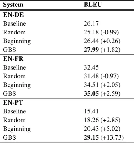
As a sanity check that improvements in BLEU are not merely due to the presence of the terms somewhere in the output, i.e. that theplacement of the terms by GBS is reasonable, we also eval-uate the results of randomly inserting terms into the baseline output, and of prepending terms to the baseline output.
This simple method of domain adaptation leads to a significant improvement in the BLEU score without any human intervention. Surprisingly, even an automatically created terminology com-bined with GBS yields performance improve-ments of approximately+2BLEU points for
En-De and En-Fr, and a gain of almost 14 points for En-Pt. The large improvement for En-Pt is probably due to the training data for this sys-tem being very different from the IT domain (see Appendix). Given the performance improve-ments from our automatically extracted terminol-ogy, manually created domain terminologies with good coverage of the test domain are likely to lead to even greater gains. Using a terminology with GBS is likely to be beneficial in any setting where the test domain is significantly different from the domain of the model’s original training data.
System BLEU
EN-DE
Baseline 26.17
Random 25.18 (-0.99)
Beginning 26.44 (+0.26)
GBS 27.99(+1.82)
EN-FR
Baseline 32.45
Random 31.48 (-0.97)
Beginning 34.51 (+2.05)
GBS 35.05(+2.59)
EN-PT
Baseline 15.41
Random 18.26 (+2.85)
Beginning 20.43 (+5.02)
[image:7.595.73.292.461.694.2]GBS 29.15(+13.73)
Table 2: BLEU Results for EN-DE, EN-FR, and EN-PT ter-minology experiments using the Autodesk Post-Editing Cor-pus. ”Random’ indicates inserting terminology constraints at random positions in the baseline translation. ”Beginning” indicates prepending constraints to baseline translations.
4.3 Analysis
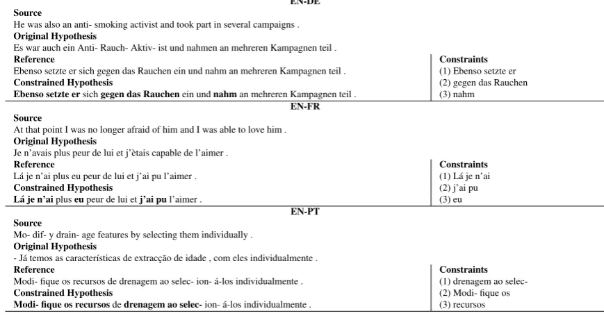
Subjective analysis of decoder output shows that phrases added as constraints are not only placed correctly within the output sequence, but also have global effects upon translation quality. This is a desirable effect for user interaction, since it im-plies that users can bootstrap quality by adding the most critical constraints (i.e. those that are most essential to the output), first. Table3shows several examples from the experiments in Table1, where the addition of lexical constraints was able to guide our NMT systems away from initially quite low-scoring hypotheses to outputs which perfectly match the reference translations.
5 Related Work
Most related work to date has presented modifica-tions of SMT systems for specific usecases which constrain MT output via auxilliary inputs. The largest body of work considers Interactive
Ma-chine Translation(IMT): an MT system searches
for the optimal target-language suffix given a com-plete source sentence and a desired prefix for the target output (Foster,2002;Barrachina et al., 2009;Green,2014). IMT can be viewed as sub-case of constrained decoding, where there is only one constraint which is guaranteed to be placed at the beginning of the output sequence. Wuebker et al. (2016) introduce prefix-decoding, which modifies the SMT beam search to first ensure that thetarget prefixis covered, and only then contin-ues to build hypotheses for the suffix using beams organized by coverage of the remaining phrases in the source segment. Wuebker et al.(2016) and Knowles and Koehn(2016) also present a simple modification of NMT models for IMT, enabling models to predict suffixes for user-supplied pre-fixes.
EN-DE Source
He was also an anti- smoking activist and took part in several campaigns .
Original Hypothesis
Es war auch ein Anti- Rauch- Aktiv- ist und nahmen an mehreren Kampagnen teil .
Reference Constraints
Ebenso setzte er sich gegen das Rauchen ein und nahm an mehreren Kampagnen teil . (1) Ebenso setzte er
Constrained Hypothesis (2) gegen das Rauchen
Ebenso setzte ersichgegen das Rauchenein undnahman mehreren Kampagnen teil . (3) nahm
EN-FR Source
At that point I was no longer afraid of him and I was able to love him .
Original Hypothesis
Je n’avais plus peur de lui et j’`etais capable de l’aimer .
Reference Constraints
L´a je n’ai plus eu peur de lui et j’ai pu l’aimer . (1) L´a je n’ai
Constrained Hypothesis (2) j’ai pu
L´a je n’aipluseupeur de lui etj’ai pul’aimer . (3) eu
EN-PT Source
Mo- dif- y drain- age features by selecting them individually .
Original Hypothesis
- J´a temos as caracter´ısticas de extracc¸˜ao de idade , com eles individualmente .
Reference Constraints
Modi- fique os recursos de drenagem ao selec- ion- ´a-los individualmente . (1) drenagem ao
selec-Constrained Hypothesis (2) Modi- fique os
[image:8.595.79.514.66.295.2]Modi- fique os recursosdedrenagem ao selec-ion- ´a-los individualmente . (3) recursos
Table 3: Manual analysis of examples from lexically constrained decoding experiments. “-” followed by whitespace indicates the internal segmentation of the translation model (see Section3.2)
only make use of constraints that match phrase boundaries, because constraints are implemented as “rules” enforcing that source phrases must be translated as the aligned target phrases that have been selected as constraints. In contrast, our ap-proach decodes at the token level, and is not de-pendent upon any explicit structure in the underly-ing model.
Domingo et al.(2016) also consider an interac-tive scenario where users first choose portions of an MT hypothesis to keep, then query for an up-dated translation which preserves these portions. The MT system decodes the source phrases which are not aligned to the user-selected phrases un-til the source sentence is fully covered. This ap-proach is similar to the system of Cheng et al., and uses the “XML input” feature in Moses (Koehn et al.,2007).
Some recent work considers the inclusion of soft lexical constraints directly into deep models for dialog generation, and special cases, such as recipe generation from a list of ingredients (Wen et al.,2015;Kiddon et al.,2016). Such constraint-aware models are complementary to our work, and could be used with GBS decoding without any change to the underlying models.
To the best of our knowledge, ours is the first work which considers general lexically con-strained decoding for any model which outputs sequences, without relying upon alignments be-tween input and output, and without using a search
organized by coverage of the input.
6 Conclusion
Lexically constrained decoding is a flexible way to incorporate arbitrary subsequences into the out-put of any model that generates outout-put sequences token-by-token. A wide spectrum of popular text generation models have this characteristic, and GBS should be straightforward to use with any model that already uses beam search.
In translation interfaces where translators can provide corrections to an existing hypothesis, these user inputs can be used as constraints, gener-ating a new output each time a user fixes an error. By simulating this scenario, we have shown that such a workflow can provide a large improvement in translation quality at each iteration.
By using a domain-specific terminology to gen-erate target-side constraints, we have shown that a general domain model can be adapted to a new domain without any retraining. Surprisingly, this simple method can lead to significant performance gains, even when the terminology is created auto-matically.
Acknowledgments
This project has received funding from Science Foundation Ireland in the ADAPT Centre for Dig-ital Content Technology (www.adaptcentre.ie) at Dublin City University funded under the SFI Re-search Centres Programme (Grant 13/RC/2106) co-funded under the European Regional Develop-ment Fund and the European Union Horizon 2020 research and innovation programme under grant agreement 645452 (QT21). We thank the anony-mous reviewers, as well as Iacer Calixto, Peyman Passban, and Henry Elder for helpful feedback on early versions of this work.
References
Dzmitry Bahdanau, Kyunghyun Cho, and Yoshua Ben-gio. 2014. Neural machine translation by jointly learning to align and translate. arXiv preprint arXiv:1409.0473.
Sergio Barrachina, Oliver Bender, Francisco Casacu-berta, Jorge Civera, Elsa Cubel, Shahram Khadivi, Antonio Lagarda, Hermann Ney, Jes´us Tom´as, En-rique Vidal, and Juan-Miguel Vilar. 2009. Sta-tistical approaches to computer-assisted transla-tion. Computational Linguistics 35(1):3–28.
https://doi.org/10.1162/coli.2008.07-055-R2-06-29.
Ondˇrej Bojar, Rajen Chatterjee, Christian Federmann, Barry Haddow, Matthias Huck, Chris Hokamp, Philipp Koehn, Varvara Logacheva, Christof Monz, Matteo Negri, Matt Post, Carolina Scarton, Lucia Specia, and Marco Turchi. 2015. Findings of the 2015 workshop on statistical machine translation. In Proceedings of the Tenth Workshop on Statisti-cal Machine Translation. Association for Compu-tational Linguistics, Lisbon, Portugal, pages 1–46.
http://aclweb.org/anthology/W15-3001.
Shanbo Cheng, Shujian Huang, Huadong Chen, Xinyu Dai, and Jiajun Chen. 2016. PRIMT: A pick-revise framework for interactive machine trans-lation. In NAACL HLT 2016, The 2016 Con-ference of the North American Chapter of the Association for Computational Linguistics: Hu-man Language Technologies, San Diego Califor-nia, USA, June 12-17, 2016. pages 1240–1249.
http://aclweb.org/anthology/N/N16/N16-1148.pdf.
David Chiang. 2007. Hierarchical phrase-based translation. Comput. Linguist. 33(2):201–228.
https://doi.org/10.1162/coli.2007.33.2.201.
Kyunghyun Cho, Bart van Merri¨enboer, C¸alar G¨ulc¸ehre, Dzmitry Bahdanau, Fethi Bougares, Hol-ger Schwenk, and Yoshua Bengio. 2014. Learning phrase representations using rnn encoder–decoder for statistical machine translation. InProceedings of
the 2014 Conference on Empirical Methods in Nat-ural Language Processing (EMNLP). Association for Computational Linguistics, Doha, Qatar, pages 1724–1734. http://www.aclweb.org/anthology/D14-1179.
Kenneth Ward Church and Patrick Hanks. 1990.
Word association norms, mutual information, and lexicography. Comput. Linguist. 16(1):22–29.
http://dl.acm.org/citation.cfm?id=89086.89095.
Josep Maria Crego, Jungi Kim, Guillaume Klein, An-abel Rebollo, Kathy Yang, Jean Senellart, Egor Akhanov, Patrice Brunelle, Aurelien Coquard, Yongchao Deng, Satoshi Enoue, Chiyo Geiss, Joshua Johanson, Ardas Khalsa, Raoum Khiari, Byeongil Ko, Catherine Kobus, Jean Lorieux, Leid-iana Martins, Dang-Chuan Nguyen, Alexandra Pri-ori, Thomas Riccardi, Natalia Segal, Christophe Ser-van, Cyril Tiquet, Bo Wang, Jin Yang, Dakun Zhang, Jing Zhou, and Peter Zoldan. 2016. Systran’s pure neural machine translation systems. CoRR
abs/1610.05540.http://arxiv.org/abs/1610.05540. Miguel Domingo, Alvaro Peris, and Francisco
Casacu-berta. 2016. Interactive-predictive translation based on multiple word-segments. Baltic J. Modern Com-puting4(2):282–291.
George F. Foster. 2002. Text Prediction for Transla-tors. Ph.D. thesis, Montreal, P.Q., Canada, Canada. AAINQ72434.
Spence Green. 2014. Mixed-Initiative Natural Lan-guage Translation. Ph.D. thesis, Stanford, CA, United States.
Chlo´e Kiddon, Luke Zettlemoyer, and Yejin Choi. 2016. Globally coherent text generation with neural checklist models. In Proceedings of the 2016 Conference on Empirical Methods in Natu-ral Language Processing, EMNLP 2016, Austin, Texas, USA, November 1-4, 2016. pages 329–339.
http://aclweb.org/anthology/D/D16/D16-1032.pdf. Rebecca Knowles and Philipp Koehn. 2016. Neural
interactive translation prediction. AMTA 2016, Vol.
page 107.
Philipp Koehn. 2009. A process study of computer-aided translation. Machine Translation23(4):241– 263. https://doi.org/10.1007/s10590-010-9076-3.
Philipp Koehn. 2010. Statistical Machine Translation. Cambridge University Press, New York, NY, USA, 1st edition.
Stroudsburg, PA, USA, ACL ’07, pages 177–180.
http://dl.acm.org/citation.cfm?id=1557769.1557821.
Franz Josef Och and Hermann Ney. 2004. The alignment template approach to statistical machine translation. Comput. Linguist. 30(4):417–449.
https://doi.org/10.1162/0891201042544884.
Judea Pearl. 1984. Heuristics: Intelligent Search Strategies for Computer Problem Solving. Addison-Wesley Longman Publishing Co., Inc., Boston, MA, USA.
Alexander Rush, Yin-Wen Chang, and Michael Collins. 2013. Optimal beam search for machine translation. In Proceedings of the 2013 Confer-ence on Empirical Methods in Natural Language Processing. Association for Computational Linguis-tics, Seattle, Washington, USA, pages 210–221.
http://www.aclweb.org/anthology/D13-1022.
Alexander M. Rush, Sumit Chopra, and Jason We-ston. 2015. A neural attention model for abstrac-tive sentence summarization. In Llus Mrquez, Chris Callison-Burch, Jian Su, Daniele Pighin, and Yuval Marton, editors,EMNLP. The Association for Com-putational Linguistics, pages 379–389.
Rico Sennrich, Barry Haddow, and Alexandra Birch. 2016. Neural machine translation of rare words with subword units. In Proceedings of the 54th Annual Meeting of the Association for Com-putational Linguistics, ACL 2016, August 7-12, 2016, Berlin, Germany, Volume 1: Long Papers.
http://aclweb.org/anthology/P/P16/P16-1162.pdf.
Iulian V. Serban, Alessandro Sordoni, Yoshua Bengio, Aaron Courville, and Joelle Pineau. 2016. Building end-to-end dialogue systems using generative hierarchical neural network models. InProceedings of the Thirtieth AAAI Conference on Artificial Intel-ligence. AAAI Press, AAAI’16, pages 3776–3783.
http://dl.acm.org/citation.cfm?id=3016387.3016435.
Jason R. Smith, Herve Saint-amand, Chris Callison-burch, Magdalena Plamada, and Adam Lopez. 2013. Dirt cheap web-scale parallel text from the common crawl. In In Proceedings of the Conference of the Association for Computational Linguistics (ACL.
Lucia Specia. 2011. Exploiting objective annotations for measuring translation post-editing effort. In Pro-ceedings of the European Association for Machine Translation. May.
Ralf Steinberger, Bruno Pouliquen, Anna Widiger, Camelia Ignat, Toma Erjavec, and Dan Tufi. 2006. The jrc-acquis: A multilingual aligned parallel cor-pus with 20+ languages. InIn Proceedings of the 5th International Conference on Language Resources and Evaluation (LREC’2006. pages 2142–2147.
Ilya Sutskever, Oriol Vinyals, and Quoc V. Le. 2014. Sequence to sequence learning with neural networks. In Proceedings of the 27th
International Conference on Neural Informa-tion Processing Systems. MIT Press, Cam-bridge, MA, USA, NIPS’14, pages 3104–3112.
http://dl.acm.org/citation.cfm?id=2969033.2969173.
Zhaopeng Tu, Yang Liu, Lifeng Shang, Xiaohua Liu, and Hang Li. 2016. Neural machine translation with reconstruction. arXiv preprint arXiv:1611.01874.
Bart van Merrinboer, Dzmitry Bahdanau, Vincent Du-moulin, Dmitriy Serdyuk, David Warde-Farley, Jan Chorowski, and Yoshua Bengio. 2015. Blocks and fuel: Frameworks for deep learning. CoRR
abs/1506.00619.
Tsung-Hsien Wen, Milica Gaˇsi´c, Nikola Mrkˇsi´c, Pei-Hao Su, David Vandyke, and Steve Young. 2015. Semantically conditioned lstm-based natural lan-guage generation for spoken dialogue systems. In Proceedings of the 2015 Conference on Em-pirical Methods in Natural Language Processing (EMNLP). Association for Computational Linguis-tics.
Yonghui Wu, Mike Schuster, Zhifeng Chen, Quoc V. Le, Mohammad Norouzi, Wolfgang Macherey, Maxim Krikun, Yuan Cao, Qin Gao, Klaus Macherey, Jeff Klingner, Apurva Shah, Melvin Johnson, Xiaobing Liu, ukasz Kaiser, Stephan Gouws, Yoshikiyo Kato, Taku Kudo, Hideto Kazawa, Keith Stevens, George Kurian, Nishant Patil, Wei Wang, Cliff Young, Jason Smith, Jason Riesa, Alex Rudnick, Oriol Vinyals, Greg Corrado, Macduff Hughes, and Jeffrey Dean. 2016. Google’s neural machine translation system: Bridging the gap between human and machine translation. CoRR
abs/1609.08144.http://arxiv.org/abs/1609.08144.
Joern Wuebker, Spence Green, John DeNero, Sasa Hasan, and Minh-Thang Luong. 2016. Models and inference for prefix-constrained machine trans-lation. In Proceedings of the 54th Annual Meet-ing of the Association for Computational LMeet-inguistics (Volume 1: Long Papers). Association for Compu-tational Linguistics, Berlin, Germany, pages 66–75.
http://www.aclweb.org/anthology/P16-1007.
Kelvin Xu, Jimmy Ba, Ryan Kiros, Kyunghyun Cho, Aaron Courville, Ruslan Salakhudinov, Rich Zemel, and Yoshua Bengio. 2015. Show, attend and tell: Neural image caption generation with visual atten-tion. In David Blei and Francis Bach, editors,
Proceedings of the 32nd International Conference on Machine Learning (ICML-15). JMLR Workshop and Conference Proceedings, pages 2048–2057.
http://jmlr.org/proceedings/papers/v37/xuc15.pdf.
Matthew D. Zeiler. 2012. ADADELTA: an adap-tive learning rate method. CoRR abs/1212.5701.
http://arxiv.org/abs/1212.5701.
A NMT System Configurations
We train all systems for 500000 iterations, with validation every 5000 steps. The best single model from validation is used in all of the experiments for a language pair. We use`2regularization on all pa-rameters withα = 1e−5. Dropout is used on the output layers withp(drop) = 0.5. We sort
mini-batches by source sentence length, and reshuffle training data after each epoch.
All systems use a bidirectional GRUs (Cho et al., 2014) to create the source representation and GRUs for the decoder transition. We use AdaDelta (Zeiler,2012) to update gradients, and clip large gradients to 1.0.
Training Configurations EN-DE
Embedding Size 300 Recurrent Layers Size 1000 Source Vocab Size 80000 Target Vocab Size 90000
Batch Size 50
EN-FR
Embedding Size 300 Recurrent Layers Size 1000 Source Vocab Size 66000 Target Vocab Size 74000
Batch Size 40
EN-PT
Embedding Size 200 Recurrent Layers Size 800 Source Vocab Size 60000 Target Vocab Size 74000
Batch Size 40
A.1 English-German
Our English-German training corpus consists of 4.4 Million segments from the Europarl (Bojar et al., 2015) and CommonCrawl (Smith et al., 2013) corpora.
A.2 English-French
Our English-French training corpus consists of 4.9 Million segments from the Europarl and Com-monCrawl corpora.
A.3 English-Portuguese
Our English-Portuguese training corpus consists of 28.5 Million segments from the Europarl,
JRC-Aquis (Steinberger et al., 2006) and OpenSubti-tles5corpora.