J. Range Manage.
55: 474-481 September 2002
Estimating soil water content in tallgrass prairie using
remote sensing
PATRICK J. STARKS AND THOMAS J. JACKSON
Authors are Soil Scientist, USDA-ARS, Grazinglands Research Laboratory, El Reno, Okla. 73036, and Hydrologist, USDA-ARS, Hydrology Laboratory, Beltsville, Md. 20705.
Abstract
Increased demand for available water supplies necessitates that tools and techniques be developed to quantify soil water reserves over large land areas as an aid in management of water resources and watersheds. Microwave remote sensing can pro- vide measurements of volumetric water content of the soil sur- face (0vSL) up to about 10 cm deep. The objective of this study was to examine the feasibility of inferring the volumetric water content of the soil profile (°vBL) by combining remotely sensed estimates of 6vSL, in situ measurements, and modeling tech- niques. A simple soil water budget model was modified to esti- mate °vBL from assimilated values of BvSL Four modeling sce- narios were evaluated at 4 tallgrass prairie sites located in cen- tral and south central Oklahoma: l) unmodified model, 2) assim- ilation of field-measured °vSL at 2-day intervals, 3) assimilation of field-measured °vSL matching dates of remote sensing data acquisitions during the study period, and 4) assimilation of remotely sensed °vSL The unmodified model (scenario 1) under- estimated measurements with root mean square errors (RMSE) between 0.03 and 0.06 m3m'3 and mean errors (ME) between 0.02 and 0.04 m3m'3. Model output from scenario 2 areed well with measurements at all study sites (IMEI 0.01 m3m , RMSE 0.03 m3m'3). The RMSE and ME values from scenario 3 were compa- rable to those of scenario 2. Simulations from scenario 4 agreed well with measured data at 2 study sites (0.00 m3m'3 ME 0.02 m3m 3, RMSE 0.03 m3m'3) but underestimated measurements at the remaining sites, in one case by as much as 0.15 m3m 3. The underestimation was due largely to inaccurate remotely sensed
°vSL values. These preliminary results suggest that it is feasible to infer °vSL in tallgrass prairies by combining remotely sensed estimates of 0vSL' in situ field measurements, and modeling, pro- vided that the remotely sensed data correctly estimates surface conditions.
Key Words: hydrology, microwave, water budget
Rangelands comprise over 60% of the land area of the 48 con- tiguous states, and agricultural, industrial, recreational, and municipal water supplies in many areas of the U.S. are linked directly to rangeland watershed management (Spaeth et al. 1996).
An important part of the water budget of any watershed is the amount of water stored in the soil. Although soil water accounts
Manuscript accepted 30 Dec. 2001.
Resumen
La creciente demanda del suministro de agua disponible nece- sita que se desarrollen herramientas y tecnicas para cuantificar las reservas de agua en el suelo en grandes extensiones como una ayuda en el manejo de los recursos de agua y las cuencas hidrologicas. Los sensores remotos de microondas pueden proveer de medidas del contenido volumetrico de la superficie (°vSL) hasta cerca de 10 cm de profundidad. El objetivo de este estudio fue examinar la factibilidad de inferir el contenido volumetrico de agua del perfil del suelo (0vBL) al combinar las estimaciones de sensores remotos de BvSL mediciones in situ y tecnicas de modelaje. Un modelo simple de las reservas de agua se modifico para estimar °vBL a partir de valores asimilados del
°vSL Se evaluaron cuatro escenarios de modelaje en cuatro sitios de pradera de zacates altos localizados en las regions cen- tral y sur-central de Oklahoma: l) El modelo sin modificaciones, 2) la asimilacion de mediciones de campo del °vSL a intervalos de 2 dias, 3) la asimilacion de mediciones de campo del °vSL con- cordantes con las fechas de adquisicion de datos de sensores remotos durante el periodo de estudio y 4) la asimilacion del
°vSL a partir de sensores remotos. El modelo sin modificar (esce- nario 1) subestimo las mediciones con la raiz de los cuadrados medios de los errores (RCME) entre 0.03 y 0.06 m3m'3 y los errores medios (EM) entre 0.02 y 0.04 m3m . El modelo resul- tante del escenario 2 concordo bien con las mediciones en todos los sitos de estudio (IEMI 0.01 m3m'3, RCME 0.03 m3m'3).
Los valores de RCME y EM del escenario 3 fueron comparables con los del escenario 2. Las simulaciones del escenario 4 concor- daron bien con los datos obtenidos en dos sitios de estudio (0.00 m3m-3 ME 0.02 m3m 3, RCME 0.03 m3m'3) pero subesti- maron las mediciones en el resto de los sitios, en un caso por tanto como 0.15 m3m'3. La subestimacion se debio en gran parte a que los valores del BvSL de los sensores remotos eran inexactos.
Estos resultados preliminares sugieren que es posible inferir el
°vSL en las praderas de pastos altos mediante la combinacion de estimaciones del °vSL obtenidas a partir de sensores remotos, mediciones de campo en el sitio y modelaje y que los datos de sensores remotos estimaron correctamente las condiciones de la superf icie.
for only about 0.0001% of the total water on earth, it is a key component in describing the transfer and distribution of mass and energy between the land surface and the atmosphere, it exerts major influences on forage and crop productivity, and it partitions rainfall into runoff and infiltration (Islam 1996). Increased
474 JOURNAL OF RANGE MANAGEMENT 55(5) September 2002
100
Little Washita River Experimental Watershed
10
0 0
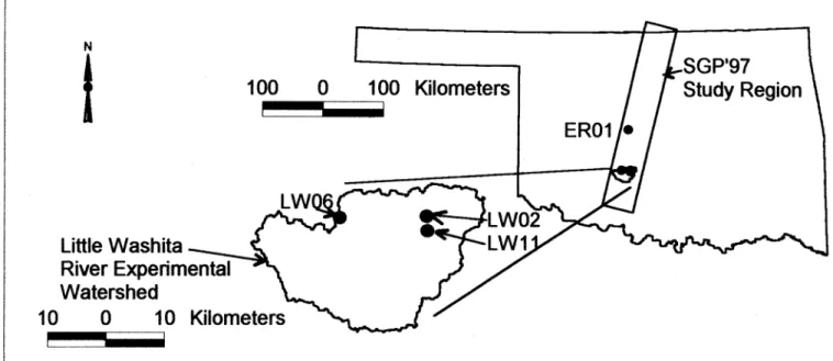
0 10 KilometersFig. 1. Study site locations within the SGP `97 study area.
demand for available water supplies necessitates that tools and techniques be developed to quantify soil water resources over large land areas, such as rangelands, as an aid in management of water resources and watersheds. Equipping watersheds with soil water content mea- surement sites for routine monitoring is impractical and expensive, especially if the watershed is large or spatially variable in its topography, soil types, and vegeta- tion cover. Remote sensing is a technique that offers potential for providing frequent measurements over large land areas in a timely and cost-effective manner.
Microwave remote sensing can provide measurements of volumetric water content (0v) up to about 10 cm deep, depending upon sensor type and wavelength used (Engman and Chauhan 1995). The Southern Great Plains 1997 Hydrology Experiment (Jackson et al. 1999), referred to herein as SGP `97, provides a recent example of attempts to use new microwave technologies to quantify sur- face soil water content (evSL) over large, spatially diverse regions at satellite spatial resolutions. One specific objective of SGP
`97, and the objective of this paper, was to examine the feasibility of inferring soil profile water content (evBL) by combining remotely sensed estimates of evSL in situ measurements, and modeling techniques (SGP 1997).
Ragab (1995) introduced a simple soil water budget model designed to incorpo- rate evSL measurements (in situ or
0
remotely sensed) to provide estimates of water content within the soil profile. The model requires basic meteorological data and easily obtained soil parameters, which makes it attractive for use in areas where little may be known about the underlying soils. The model was evaluated at 2 short grass pasture sites in England, and found to produce satisfactory results for those conditions (Ragab 1995), but the model was not used with remotely sensed data as input.
In this paper, remotely sensed OvSL and in situ measurements are combined in Ragab's model to estimate evBL to a depth of 60 cm. First, the original model's abili- ty to reproduce measured time series of
evBL is evaluated using measured meteo- rological, soil, and vegetation conditions at 4 experimental sites within the study area and period (18 June-16 July 1997) of the SGP `97 experiment.
Model simulations tend to drift because numerical algorithms are simplifications of complex physical processes. Because of this drift, data assimilation techniques may be employed whereby measured data are incorporated into the model to initialize or constrain the model to produce more real- istic simulations. Applications of data assimilation arose within the meteorologi- cal community (Daley 1991), but the application of these techniques to remote sensing and soil water modeling is rela- tively new (e.g., Calvet et al. 1998, Houser et al. 1998, Wigneron et al. 1999a, 1999b;
Hoeben and Troch 2000, Walker et al.
2001). A number of data assimilation tech- niques exist and they vary in complexity (Walker et al. 2001). The direct insertion technique is used herein to determine if assimilation of frequent, regularly-spaced field measurements of evSL improves model estimations of evBL compared to that provided by the original model. Next, the effect of assimilating field-measured evSL at irregular intervals is assessed.
Lastly, remotely sensed estimates of 0vSL are assimilated into the model to detect the effects of remotely sensed observations of
evSL on model estimates of evBL'
Materials and Methods
Site Descriptions
Four study sites within the SGP `97 experimental area were chosen for model evaluation. Three of the sites (LW02, LW06, LW 11) were located on ARS' Little Washita River Experimental Watershed (LWREW), near Chickasha, Okla. (Lat. 34° 53' Long. 98° 07'), and one (ERO 1) was located at ARS's Grazing- lands Research Laboratory near El Reno, Okla. (Fig. 1). All of these sites were clas- sified as native grassland (SGP 1997) and were dominated by big bluestem (Andropogon gerardii Vitman), little bluestem (Schizachyrium scoparium
(Michx.) Nash), indiangrass (Sorghastrum
nutans (L.) Nash) and switchgrass (Panicum virgatum L.). Despite similari-
Table 1. Leaf area index (LA!) and biomass measurements for the study sites. These data were taken from Hollinger and Daughtry (1999).
Site LAI Green Standing Biomass Standing Biomass Surface Residue (Litter) Wet Dry Water
Content
Dry Dry
Content ----(gm `)---- -(%-)- ----(gm 2)---- 2)---- -
EROI 4.7 1403 460 97 510
LWO2 2.2 350 161 158 141
LWO6 0.9 112 41 18 12
LW11 3.6 940 246 44 319
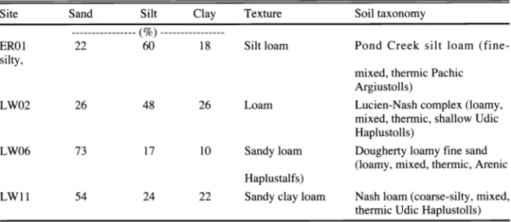
Table 2. Soil particle fractions and texture of the soil profile and taxonomy of the soils for each site.
Site Sand Silt taxonomy
ERO1 22 60 loam Creek silt loam (fine-
silty,
LWO2 6 8 6
thermic Pachic Argiustolls)
Lucien-Nash complex (loamy,
LWO6 73 17 loam
thermic, shallow Udic Haplustolls)
Dougherty loamy fine sand
LW 11 54 24 Sandy clay loam loam mixed,
thermic Udic Haplustolls)
ties in species composition, Hollinger and Daughtry (1999) showed that other vege- tation conditions varied widely between sites during the study period. For example, the leaf area index at ERO1 was 4.7, while that at LWO6 was 0.9. Additionally, litter mass at ERO1 measured 510 g m 2 (on a dry matter basis), which is about 1.5 times that measured at site LW 11 and 42 times that at LWO6 (Table 1).
The soil profile at each site was sampled to a depth of 60 cm in 15 cm depth inter- vals using a coring tool with a 5 cm inside diameter. Depth intervals were divided into 7.5 cm long sub-samples. One sub- sample was used to determine soil texture using the hydrometer method (Day 1965).
Soil texture for the total soil profile was
calculated as the average of the sand, silt, and clay fractions of the four subsamples (Table 2). The remaining sub-sample was used to determine the soil water release curve at each depth interval using the pro- cedure given in Ahuja et al. (1985). Soil water release curves allow conversion of soil matric potential (ip), the measure of the soil matrix capillary and absorptive forces exerted on water, into estimates of 0v. Laboratory determination of the soil water release curves provided direct mea- surement of bulk density and the required model parameters of 8v at saturation
(0vS), field capacity (0vFC)' and wilting point (6vWp) (Table 3).
Table 3. Surface (0.5cm) and soil profile (0.60cm) volumetric soil water contents (8v) at field capacity (FC), wilting point (WP) and saturation (S) used in the model.
Site Layer evFC
3 3
ERO1 Surface 0.32
Soil profile 0.32 0.24
LWO2 Surface 0.32
Soil profile 0.31 0.11
LWO6 Surface 0.17
Soil profile 0.17 0.02
LW11 Surface 0.29
Soil profile 0.29 0.06
Meteorological and 8v Field Measurements
Air temperature, rainfall, relative humidity, wind speed, incoming solar radiation, and barometric pressure were recorded at meteorological stations located at or near each study site. These data were used in a Penman-Monteith equation to calculate potential ET (ET) at sites LWO6 and LW 11. Actual ET (ETa) was calculat- ed at sites ERO1 and LWO2 using the Bowen ratio/energy balance approach (Rosenberg et al. 1983).
A Soil Heat and Water Measurement System (SHAWMS) was installed at each of the 4 sites prior to SGP `97. Each SHAWMS was placed inside a fenced enclosure measuring about 3.7 m on a side and about 1.3 m high. The vegetation within the enclosure was monitored regu- larly and managed to match surrounding field conditions as closely as possible. The SHAWMS instrumentation includes soil heat dissipation sensors (HDS) (Model 229, 'Campbell Scientific, Inc., Logan, Utah) which provided hourly measure- ments of ip with 3 replications at 5 cm and
1 replication each at 10, 15, 20, 25, and 60 cm below the soil surface. All HDSs were calibrated according to the method out- lined in Starks (1999). Conversion of ip to 8v was based on the site- and depth-spe-
cific soil water release curves. The SHAWMS HDS output at 1200 hours (CST) was used to represent daily 0v since it was nearly co-incident with the time that the remotely sensed data were obtained over the area. Measured 6vBL was calcu- lated as a weighted average of the HDS readings.
Elliott et al. (1999), Humes et al. (1999), Schneider et al. (1999), and Starks et al.
(1999) found good correspondence between ev derived from HDSs and gravi- metrically-based values, and to values obtained from various types of electronic sensors. The HDS-derived 6v tended to overestimate gravimetrically obtained val- ues by about 0.02 m3m 3, on average, at 3
study sites in Oklahoma (Starks 1999).
When a sandy site was eliminated from the analysis, the overestimation was <_
0.01 m3m 3. Humes (personal communica- tion) compared ev derived from both HDS and that determined gravimetrically from soil cores at a number of locations in Oklahoma and found that the HDS values
Names are necessary to report factually on avail- able data; however, the USDA neither guarantees or warrants the standard of the product, and the use of the name by the USDA implies no approval of the product to the exclusion of others that may also be suitable.
476 JOURNAL OF RANGE MANAGEMENT 55(5) September 2002
were within about 0.05 m3m 3 of those obtained from the soil cores.
The HDSs tend to lose hydraulic contact with sandy soils and do not yield consis- tently reliable data under those conditions (Starks 1999). Therefore, at sites LW06 and LW11, gravimetric and time-domain reflectometry (TDR) measurements were used to determine evSL and BvBL' respec- tively. The TDR measurements at these 2 sites were obtained daily (weather permit- ting) during the 16 June-18 July experi- mental period within 2 hours of the remotely sensed data. An Environmental Sensors' MoisturePoint TDR (G.S. Gabel Corporation, British Columbia, Canada), utilizing 4-segment profiling rods, was used to sample the soil profile at 0-15, 15-30, 30-45 and 45-60 cm. Three read- ings were acquired per site per layer and were averaged to represent daily °VBL' The manufacturer's stated accuracy of the TDR is ± 3% of the instrument reading.
Nine soil samples, representing the 0-5 cm surface layer, were collected once daily over a 20 m by 20 m grid at each site. Gravimetric soil water content was determined for each sample, averaged and multiplied by the respective soil's bulk density to obtain a representative value of
BvSL for each site. Standard deviations of the gravimetric soil water contents ranged between 0.01 and 0.04 m3m 3.
Remotely Sensed Data
Remotely sensed images of surface microwave brightness temperatures (TB) were acquired over the 10,000 km2 SGP
`97 study area using the Electronically Scanned Thinned Array Radiometer
(ESTAR). The ESTAR is an L band, syn-
thetic aperture, passive microwave
radiometer operating at a center frequency of 1.413 GHz (21 cm) and a bandwidth of 20 MHz. The ESTAR instrument was flown onboard a NASA P3B aircraft at an altitude of 7.5 km. Postprocessing of the remotely sensed data produced a pixel size of 800 m by 800 m. Because of weather conditions and equipment failures, the ESTAR was only able to collect data on 16 days of the 29 day study period.
Nominal time over target was 0930 to 1130 hours local time.
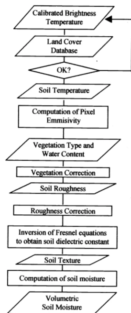
Brightness temperatures measured by ESTAR are affected by a number of sur- face conditions which must be taken into account before a final BvSL can be deter- mined. Figure 2 is a diagram of the soil moisture retrieval algorithm used to con- vert TB to evSL Input requirements for the model are soil temperature at 15 cm, vegetation type, vegetation water content,
soil roughness, and soil texture. The model corrects TB for vegetation cover and surface roughness, and then estimates the soil's dielectric constant. Soil texture effects are then taken into account before inverting the dielectric mixing model (Wang and Schmugge 1980) to provide the final remote sensing images of evSL' For additional details of the soil moisture algorithm see Jackson (1993).
Study site latitude and longitude coor- diates were used in an image processing system to locate and extract evSL values from the ESTAR images, which were sub- sequently assimilated into the model.
The Model
The model is a one-dimensional soil water budget algorithm based on the force-restore concept presented by Bhumralkar (1975) for soil temperature, later adapted to soil water movement by Deardorff (1977). The model is divided into a surface layer (the remote sensing depth, 0-5 cm for this study) and a layer that extends from the soil surface to a user-defined depth (termed bulk layer by Ragab). In the remainder of this paper the term bulk layer will be used in preference to soil profile.
The model operates on a daily time step and the required meteorological data are daily values of rainfall and ET. The ETp values are adjusted within the model by a stress factor to estimate ETa. The stress factor is the ratio of actual available to maximum available soil water content.
The model was modified to bypass the stress adjustment when measured ETa val- ues are used. Required soil parameters include depth of the surface and bulk lay- ers; and, for each layer, evFC (0v corre- sponding to ip of -33 kPa ), °VWp (0v cor- responding to ip of -1500 kPa), antecedent ev (initial soil water content at the begin- ning of the model run), and maximum and minimum model-allowed ev (prevents model estimates from being unrealistically wet or dry). The user can partition a por- tion of incident rainfall into runoff through the "surface runoff percentage" variable.
This variable is initialized at the beginning of the model run and all subsequent rain- fall events are partitioned in the same fashion. Since most rainfall events that occurred in this study were light, this van- able was set to zero (i.e., no runoff). The
"uptake ratio" variable is used to define the surface layer's contribution to ETa. In this study the uptake ratio was set to 0.25 at all sites.
Dynamically, evSL is determined as a function of rainfall, runoff, ETa, and the
Calibrated Brightness Temperature
Land Cover Database
Soil Temperature
I
Computation of Pixel Emmisivity
Vegetation Type and Water Content
I Vegetation Correction Soil Roughness
L Roughness Correction 7
Inversion of Fresnel equations to obtain soil dielectric constant
Soil Textur
1
Computation of soil moisture
Volumetric Soil Moisture
Fig. 2. Schematic of the soil moisture retrieval algorithm (adapted from Jackson, 1993).
amount of water in the bulk layer. The rate of exchange of water between the surface and bulk layer is governed by a pseudo- diffusivity coefficient (C), which depends upon surface soil texture and BvBL The value of C at our four study sites was empirically determined by running the model at sites with similar soils and mak- ing adjustments to C until the best match between model output and measured data was achieved.
Calculation of 6vBL is independent of surface layer computations and is a simple water budget requiring only daily values of rainfall, runoff, and ET. Thus, assimila- tion of surface BvSL measurements into the original model will not affect bulk layer calculations. Therefore the original model was re-written in order that mea- surements of evSL could be assimilated into the model to infer evBL To this end, we adapted the statistical procedure out- lined in Ragab (1995) for determining model initialization values for the bulk layer from surface measurements. This procedure utilizes site-specific linear regression equations, developed from field
i
Table 4. Slope, intercept and coefficient of determination (r2) of linear regression equa- tions used to convert remotely sensed surface 6v to root zone soil water storage (mm). Root zone soil water storage is divided by depth of the root zone to estimate root zone 6.
Site slope intercept
EROI 387.76 67.13
LW02 309.58 67.02 LW06 409.96 43.21
LW11 307.96 86.33
measurements, which relate 6VSL (in m3m 3) to the depth of water stored (in mm) in the bulk layer. Soil water storage values from the regression equations are divided by the bulk layer depth to yield updated values of BvBLCorrelation coefficients from the linear regressions (Table 4) are similar to those reported by Ragab (1995) for 2 soils in southern England.
The model was run for 4 scenarios. The
first scenario examines the original model's ability to simulate °VBL for the meteorologic, soil, and vegetation condi- tions at each of the study sites. In this sce- nario the initial °vBL values are supplied from field-measured data. The model then produces a time series of °vBL based only upon the meteorological drivers of rainfall and ETa and the measured soil and vegeta-
0.45 0.40 0.35 0.30 0.25 0.20 0.15 0.10 0.05 0.00
IAD ;: h h Or0
ER01
A
a0
Day of Year
LWn6
O 00 Co oN. I. h n h O M
Day of Year
- IinfatI (mm) Measured
-fr-Scenario 2 -s-Scenario 3
tion parameters initially supplied to the model. In the second scenario, field mea- surements of BvSL are assimilated into the model at 2-day intervals to determine if model simulations of °vBL are improved over that of scenario 1. The 2-day interval was chosen in response to the frequency of surface soil moisture products that may become available on future satellite plat- forms. For example, the European Space Agency's ENVISAT has a primary repeat coverage cycle of 35 days, but will have coverage subcycles of 1, 3, and 17 days (http://envisat.esa.intl accessed 7 Jan.
2002). In scenario 3, field measurements are again used to update the model but only on those days corresponding to the times when the ESTAR was used to col- lect data during the study period. Since the ESTAR did not fly every day during the study period, this scenario examines the effect of irregular and/or infrequent data assimilation on model simulations during the study period. In the fourth scenario, ESTAR data, which represents a 800 m by 800 m spatial average of 6vSL' are assimi- lated into the model.
Statistical Analysis
Willmott and Wicks (1980) and Willmott (1981, 1982) raised concerns
t
r r + 20
+10
0) i- M m F.
r r r % N r
0~0 eb C 01 0)
-Scenario 1
-f-Scenario 4
m r a Co r r . r p.- e r U) M a) r H a1 r P a .- r
Day of Year (1997) w r
M a r
a M as
Fig. 3. Time series plots of measured and modeled bulk layer volumetric soil water content for study sites ERO1 (a), LW02 (b), LW06 (c) , and LWII (d) during the experimental period. Gaps in the time series reflect days when measured values were unavailable for comparison with modeled out- put.
about the exclusive use of r and r2 in the context of evaluating model performance.
Willmott (1981) noted that very dissimilar values of measurements and estimates can produce an r very near 1, while small dif- ferences between measured and estimated quantities can produce a low or even nega- tive r (Willmott and Wicks 1980).
Willmott (1982) proposed the d-index of model agreement which, when used in conjunction with other common statistical measures, aids in evaluating the accuracy of models. A d = 1 indicates complete agreement between modeled and mea- sured values, and d = 0 indicates complete disagreement. The d-index is used herein to evaluate how well model output agrees with measured field data for each of the 4 scenarios. In addition, the mean error (ME) and root mean square error (RMSE) were used to describe the average differ- ence between modeled and measured val- ues and to describe the average total error in the estimating procedure, respectively.
A no-intercept linear regression analysis was used to determine r2 and regression coefficients (slope, designated iii) between measured and modeled values. A t-test was used to determine if the modeled values are significantly different from measured values by testing the null hypothesis, Ho: R i =1. Preliminary analy-
a0 00 Op U)
r r r r r r
Day of Year (1997)
LW11
r r h
478 JOURNAL OF RANGE MANAGEMENT 55(5) September 2002
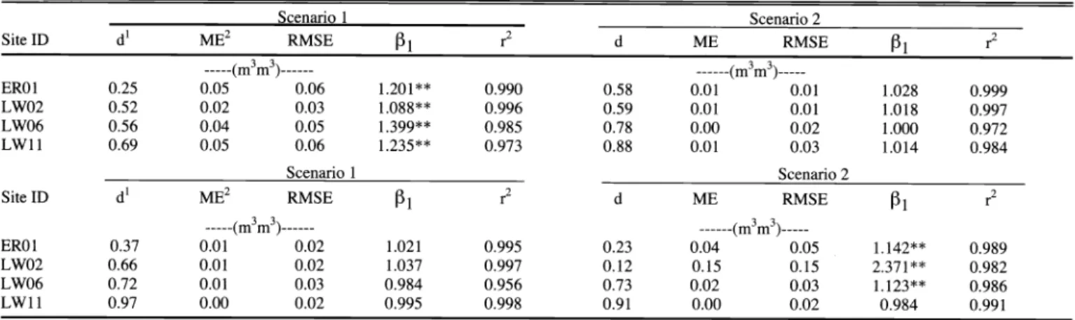
Table 5. Results from the statistical analysis of the comparison of modeled and measured bulk layer soil water content for each scenario.
Scenario 1 Scenario 2
Site ID di
ME2 1 d
3 3 3 3
---(m m)--- ---(m m)---
EROI 0.25 0.05 0.01
LWO2 0.01
LWO6 0.00
LW 11 0.05 0.03
1 Scenario 2
RMSE d ME RMSE
3 3 3 3
0.01 0.23 0.04 0.05 1.142** 0.989
LWO2 0.66 0.01 0.02 1.037 0.997 0.12 0.15 0.15 2.371** 0.982
LWO6 0.72 0.01 0.03 0.984 0.956 0.73 0.02 0.03 1.123** 0.986
LW 11 0.97 0.00 0.02 0.995 0.998 0.91 0.00 0.02 0.984 0.991
**significant at the 0.01 level
'd =1- [(Modeled - Measured)2I(IModeled - Mean of Measuredl2 + (Measured - Mean of Measuredl2)]
2ME = (Measured - Modeled) I n 3RMSE = [(Modeled - Measured)2In]ll2
sis showed that the residual lack of fit in the no-intercept regression analyses was small and not a realistic estimate of the true error because of the extremely good fit of the model output to the measured data. Thus, an error of 0.03 m3m 3 in the HDS and TDR measurements is assumed and is used as an approximation of the standard error of the estimate in the t- equation. Since the study objective relates to the bulk layer, only the results from that layer are reported.
Results
Scenario 1- Original Model
The range of measured 0VBL over the course of the study period was about 0.04 m3m 3 at sites ERO1 and LWO2, 0.08 m3m 3 at LWO6, and 0.14 m3m3 at LW11. These ranges of measured evBL represent 50, 20, 93, and 61% of the total plant available water (defined as the difference in water content at field capacity and wilting point) at these sites, respectively. Time series simulations from the original model exhib- it the general patterns portrayed by the measured data, but the model consistently underestimated measured values at all sites (Figs. 3a-3d). The differences
between measured and modeled BvBL gen- erally increase with time at sites ERO1 and LWO2, while at sites LWO6 and LW 11
there appears to be a constant offset or bias in the model simulations (Figs.
3a-3d).
The r2 values indicate that the variation in the modeled values is strongly associat- ed with the variation in the measurements at all sites (Table 5), but the i 1 are signifi- cantly different from a slope of 1, indicat- ing that the modeled output does not
approximate measured values well. The d- index (Table 5), however, indicates weak agreement between measured and mod- eled values at ERO1, moderate agreement at sites LWO2 and LWO6, and stronger agreement at LW 11. The ME reveals that the model underestimated measured val- ues from 0.02 m3m 3 at site LWO2 to 0.05 m3m 3 at site ERO1. Only site LWO2 had a RMSE <_ 0.05 m3m 3
Scenario 2
Assimilation of field-measured 6vSL values into the model at frequent, evenly- spaced intervals brings the model esti- mates of BvBL into close agreement with measured values (Figs. 3a-3d). Neither the steadily increasing differences or constant offset from measured values noted in the simulations of scenario 1 is observed here.
The d-index increased at all sites, with the greatest improvement observed at ERO1.
At all study sites, the RMSE were <_ 0.03 m3m3, a two-fold reduction at each site compared to scenario 1 (Table 5). The absolute values of ME were all <_ 0.01 m3m 3, a reduction of at least 0.04 m3m 3 at all sites, except at LWO2 where the ME was reduced by 0.01 m3m 3. The (31 values at all sites were not significantly different from a slope of 1, indicating that the model output closely approximates the measured values.
Scenario 3
Assimilation of field-measured 6vSL into the model at irregular intervals produced mixed results. At site EROI, the d-index decreased considerably in comparison to scenario 2, although the ME remained unchanged and the RMSE increased by only 0.01 mini 3 to 0.02 m3m 3 (Table 5).
Comparison of the time series plots (Fig.
3a) shows that scenarios 2 and 3 produced similar output except during consecutive days when assimilation data were unavail- able (DOY 172-175, 185-191). At site LWO2, the d-index increased slightly over
that observed in scenario 2, the ME remained unchanged and the RMSE increased by 0.01 m3m 3. The largest dis- crepancies between measured and mod- eled data at site LWO2 occurred during the 7 days from DOY 185-191 (Fig. 3b) when field measurements of 6vSL were not available to the model. The effect of assimilating evSL data at irregular inter- vals had a small negative effect at site LWO6 (Fig. 3c) as indicated by a slight decrease in the d-index and an increase of 0.01 m3m 3 in the ME and RMSE (Table 5) over that observed in scenario 2. At site LW11(Fig. 3d) the d-index (Table 5) indi- cates near-perfect agreement between modeled and measured values.
Additionally, the ME and RMSE decreased by 0.01 m3m 3 from those observed in scenario 2. It should be noted that the statistical analysis from this sce- nario shows improved simulations at all sites over that obtained in scenario 1; all d-indices are larger and all ME and RMSE values smaller than their counterparts in scenario 1. As in scenario 2, the i 1 values
were found to be statistically similar to a slope of 1.
Scenario 4
Model output at sites EROI and LWO2 did not agree well with measured data (d- index <_ 0.23) (Figures 3a-d, Table 5). At site EROI, both the ME and RMSE increased by 0.03 m3m 3 over that observed in scenario 3. Regression coeffi- cients at these 2 sites are statistically dif- ferent from a slope of 1, suggesting that