Principal component analysis aided statistical process optimisation (PASPO) for process improvement in industrial refineries

Principal component analysis-aided

statistical process optimisation (PASPO)

for process improvement in industrial

refineries

Teng, Sin Yong and How, Bing Shen and Leong, Wei Dong

and Teoh, Jun Hao and Cheah, Adrian Chee Siang and

Motavasel, Zahra and Lam, Hon Loong

Brno University of Technology, Swimburne University of Technology,

The University of Nottingham Malaysia Campus

10 July 2019

Accepted Manuscript

Principal component analysis-aided statistical process optimisation (PASPO) for process improvement in industrial refineries

Sin Yong Teng, Bing Shen How, Wei Dong Leong, Jun Hao Teoh, Adrian Chee Siang Cheah, Zahra Motavasel, Hon Loong Lam

PII: S0959-6526(19)30982-5

DOI: https://doi.org/10.1016/j.jclepro.2019.03.272

Reference: JCLP 16276

To appear in: Journal of Cleaner Production

Received Date: 26 August 2018 Revised Date: 27 February 2019 Accepted Date: 25 March 2019

Please cite this article as: Teng SY, How BS, Leong WD, Teoh JH, Siang Cheah AC, Motavasel Z, Lam HL, Principal component analysis-aided statistical process optimisation (PASPO) for process improvement in industrial refineries, Journal of Cleaner Production (2019), doi: https://doi.org/10.1016/ j.jclepro.2019.03.272.

M

A

NUS

C

R

IP

T

A

C

C

E

P

TE

M

A

NUS

C

R

IP

T

A

C

C

E

P

TE

D

Principal Component Analysis-aided Statistical Process

Optimisation (PASPO) for Process Improvement in Industrial

Refineries

Sin Yong Tenga, Bing Shen Howb, Wei Dong Leongc, Jun Hao Teohc, Adrian Chee Siang Cheahc, Zahra Motavaselc, Hon Loong Lamc,*

a_{Brno University of Technology, Institute of Process Engineering & NETME}

Centre, Technicka 2896/2, 616 69 Brno, Czech Republic

b_{Chemical Engineering Department, Faculty of Engineering, Computing and}

Science, Swinburne University of Technology, Jalan Simpang Tiga, 93350 Kuching, Sarawak Malaysia.

c_{Department of Chemical and Environmental Engineering, University of}

Nottingham Malaysia Campus, Jalan Broga, 43500 Semenyih, Selangor, Malaysia.

*Corresponding author: [email protected]

Abstract:

M

A

NUS

C

R

IP

T

A

C

C

E

P

TE

D

Keyword: Principal Component Analysis, Design of Experiment, Plant-wide Optimisation, Statistical Process Optimization, PASPO, Big Data Analytics

1.0 Introduction

Development of manufacturing plants is closely correlated with global warming, resource depletion, rising threats in food, water and energy securities and other widespread environmental risks (Wang et al., 2017). Global manufacturing environmental consequences have urged the development of cleaner and sustainable manufacturing processes (Klemes et al., 2012). The concept of sustainable development has been targeted to achieve present needs without compromising future development in the Brundtland report (WCED, 1987). Various researchers have reported that adopting the concept of green and sustainable manufacturing can lead to a significant improvement in overall performances (Lam et al., 2016). The current research paradigm has shifted to cope with the rising demand and awareness in attaining sustainable goals (Wan Alwi et al., 2014). Porter and Linde (1995) provided excellent resource conservation cases for which the “Lean and Green” strategy was adopted. The main objective of lean is to eliminate non-value-added product (Leong et al., 2018). Green, on the other hand, represents ecological sustainability which encompasses various environmental concerns, including waste generation and recycling, air, water and land pollution, energy usage and efficiency (Bhattacharya et al., 2011).

The oil and gas industry (Atanas et al., 2016), palm industry (Huda et al., 2018), and other industries have started to convert into a lean and green business model. Alsayigh (2015) performed a study on the implementation of lean and green management in oil and gas operation. Green and lean tools such as Value Stream Mapping and SWOT analysis were utilised to improve the Gulf state’s oil and gas operation energy and emission (Alsayigh, 2015). Furthermore, lean tools such as Deming’s Cycle can be used to optimise drill rig movement operation (Atanas et al., 2016). The implementation has successfully reduced process defects, improved team communication and developed efficient and robust process maps for operation. Amminudin et al. (2011), on the other hand, has successfully improved the propane recovery in Khurais central processing gas plant by conducting root cause analysis.

M

A

NUS

C

R

IP

T

A

C

C

E

P

TE

D

requires 912 discrete variables and 5599 equations. In addition, many industry players tend to increase production capacity due to surges in market demand without careful and in-depth analysis of the equipment’s capability and efficiency (Halvorsen et al., 2012). Inevitably, operating conditions deviates from optimal, process efficiency declines, and environmental performances are subpar coupling with deteriorating product quality.

The statistical approach is one of the simple yet effective ways to address all the mentioned issues. Notably, Design of Experiments (DoE) was first invented by Fisher (1935). The underlying principle is simply such that a sequence of test whereby intentional adjustment is made towards process variables and responses from the process are measured (Fisher, 1935). It can measure all correlations between process variables and responses by varying them simultaneously instead of individually. The process variables and responses are fitted in a mathematical model that used to effectively accelerate the optimisation (Toyota et al., 2017). DoE can also generate a predictive model for a great number of variables with a minimum experimental run (Gunst and Mason, 2009). Nevertheless, it is not practical for a complex problem which contains an extensive number of variables. In such problems, the required resources demand and computational time will increase exponentially with the increasing number of variables within the problem boundary (Telford, 2007). This weakness has become apparent when DoE is being applied in problems related to Big Data (Drovandi et al., 2017). With growing needs for Big Data analytics in industries including chemicals, energy, semiconductors, pharmaceuticals and food (Chiang et al., 2017), DoE becomes impracticable.

Fortunately, it is possible to prioritise the number of variables within a problem boundary through a multivariate statistical approach, called

Principal Component Analysis (PCA). In brief, Hostelling (1933) formalised

M

A

NUS

C

R

IP

T

A

C

C

E

P

TE

D

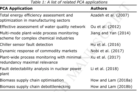
reduced computational load and efficiency. Some other reported PCA applications are tabulated in Table 1. Despite the natures of these works being different, the motives for using PCA are certainly identical (i.e., to reduce the dimensionality of the research problem without losing too much information).

Table 1: A list of related PCA applications

PCA Application Authors

Total energy efficiency assessment and optimization in manufacturing sectors

Azadeh et al. (2007)

Effective assessment of water quality network Ou et al. (2012)

Multi-mode plant-wide process monitoring scheme for complex chemical industries

Jiang and Yan (2014)

Chiller sensor fault detection Hu et al. (2016)

Dynamic response of commodity markets Nobi et al. (2017)

Plant-wide process monitoring with minimal redundancy maximal relevance

Xu et al. (2017)

Fault detectability analysis in nuclear power plant

Li et al. (2018)

Biomass supply chain optimisation How and Lam (2018a)

Biomass supply chain debottlenecking How and Lam (2018b)

M

A

NUS

C

R

IP

T

A

C

C

E

P

TE

D

19 factors, which also reduced the number of experiments from 51.2 million to 6400. Furthermore, PCA and DoE have been utilised for the optimisation of a turning unit in the works of Madhavi et al. (2017). In which, the operating conditions of a single turning unit are optimised to give optimal product hardness and surface roughness.

All the reviewed works are admirable, however, none of them has tested the capability and applicability of the proposed method with the validation in a real chemical plant for plant-wide optimisation. This paper implements a novel usage of PCA and DOE that is formulated specifically for plant-wide optimization, called the Principal Component Analysis-aided Statistical Process Optimisation (PASPO). The novel PASPO framework reduces the dimensionality of the plant-wide optimization by screening computed correlation-based principal components while decoupling and recombining the principal components into process variables for critical variable selection. This paper also demonstrates the effectiveness of the PASPO framework by using an actual industrial processing plant as a case study. The PASPO framework is aimed to reduce analysis time and cost, minimise process changes required for a relatively good benefit while making plant-wide optimisation more data-oriented (instead of model-oriented). Furthermore, environmental impact analysis is carried out to study the environmental performance of the process. To achieve this, a performance indicator known as Process Cycle Assessment (a simplification of Life Cycle Analysis (LCA) to target process systems) is developed to allow instant and effortless assessment of environmental performance.

2.0 Methodology

M

A

NUS

C

R

IP

T

A

C

C

E

P

TE

D

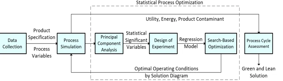
ensuring that product quality meets the requirement and environmental performance is improved (see Figure 1). The optimal operating conditions can then be plotted in a solution diagram to show its desirability and its relativeness with the high and low limits. The newly established optimum operating conditions are tested out by Process Cycle Assessment to further analyse the environmental performances.

Figure 1: Overall proposed methodology for PCA-aided statistical process optimisation (PASPO)

The overall strategies are as below:

1. Analyse the process and plan data collection strategy

2. Data is collected for all unit operations such as operating conditions, equipment capacity and safety limits

3. The process is modelled using appropriate process simulation tool (Aspen HYSYS)

4. PCA is performed to reduce the dimensions of data

5. DoE is performed to generate a regression model

6. The regression model is used to plot a surface response curve

7. Surface response plots are utilised to visualise the regression model and study the relations between process variables.

8. Numerical optimisation is used to find an optimal operating condition that would maximise yields and quality.

M

A

NUS

C

R

IP

T

A

C

C

E

P

TE

D

10.Optimised operating conditions is inputted into the simulated process model in step 3

11.Product quality before and after statistical optimisation are compared

12.Process Cycle Assessment is performed to evaluate the environmental performance of the process (before and after statistical process optimisation)

The detailed methodology for each strategy is demonstrated based on the Pentas Flora case study (introduced in Section 2.0) in the subsections below.

3.0 Case Study

M

A

NUS

C

R

IP

T

A

C

C

E

P

TE

D

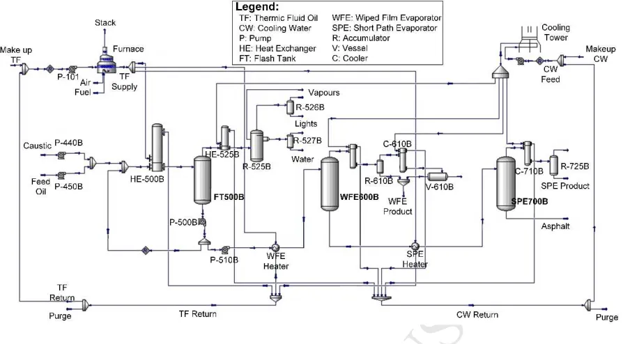
Figure 2: Simplified block flow diagram of oil re-refining case study

3.1 Data Collection

Data of the process is collected systematically to ensure all the potential correlations between the operating conditions and the responses are captured by the model. Therefore, this section presents the data collection step of this work. There are two sections of data collection, i.e., operating conditions and product specifications.

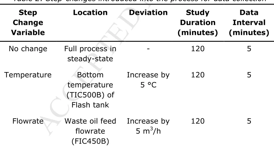
The steady-state operating conditions of all equipment in the process (e.g. temperature, pressure and flowrate) were recorded for 120 minutes with 5 minutes’ interval. Step-changes are introduced towards the process to determine the significances of all operating parameters by calculating their covariance within the PCA study (see Table 2). Likewise, the operating conditions of all equipment are extracted after the introduction of step-changes for a time span of 2 hours with 5 minutes’ interval.

Table 2: Step-changes introduced into the process for data collection

Step Change Variable

Location Deviation Study

Duration (minutes)

Data Interval (minutes)

No change Full process in steady-state

- 120 5

Temperature Bottom temperature (TIC500B) of Flash tank

Increase by 5 °C

120 5

Flowrate Waste oil feed flowrate (FIC450B)

Increase by 5 m3/h

120 5

M

A

NUS

C

R

IP

T

A

C

C

E

P

TE

D

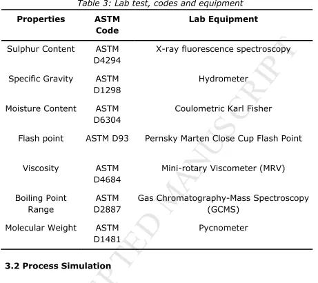
to determine the properties of oil with appropriate standards and equipment as shown in Table 3.

Table 3: Lab test, codes and equipment

Properties ASTM

Code

Lab Equipment

Sulphur Content ASTM D4294

X-ray fluorescence spectroscopy

Specific Gravity ASTM D1298

Hydrometer

Moisture Content ASTM D6304

Coulometric Karl Fisher

Flash point ASTM D93 Pernsky Marten Close Cup Flash Point

Viscosity ASTM D4684

Mini-rotary Viscometer (MRV)

Boiling Point Range

ASTM D2887

Gas Chromatography-Mass Spectroscopy (GCMS)

Molecular Weight ASTM D1481

Pycnometer

3.2 Process Simulation

Process simulation is carried out using HYSYS V8.8. The fluid package chosen is Sour Peng-Robinson (Sour PR) as it provides a good estimation for hydrocarbons and process consisting of hydrogen sulphide (H2S) contaminant (Aspen Process Engineering Webinar, 2006). The waste oil feed is then modelled using an oil blend function, while its accuracy is further enhanced by incorporating bulk properties of waste oil and boiling point range (BPR) identified from lab testing as shown in Table 4.

Table 4: Bulk Properties and boiling point range of waste feed oil

Oil Sample Feed oil

M

A

NUS

C

R

IP

T

A

C

C

E

P

TE

D

Moisture content (% w/w) 14.27

Sulphur content (ppm) 4719.70

Boiling point range

Initial Boiling Point (IBP) 133°C

10%Vol. 141°C

20%Vol. 182°C

30%Vol. 236°C

40%Vol. 286°C

50%Vol. 326°C

60%Vol. 353°C

70%Vol. 373°C

80%Vol. 399°C

90%Vol. 450°C

Final Boiling Point (FBP) 546°C

M

A

NUS

C

R

IP

T

A

C

C

E

P

TE

D

Figure 3: Simulation process flow diagram (main processing units in bold)

Table 5: Comparison between simulated and actual product specification

Oil Product

Kinematic Viscosity (cSt) Density (kg/m3)

Simulated Actual Deviation (%)

Simulated Actual Deviation (%)

WFE Product

16.82 15.37 9.43 891.5 848.7 5.04

SPE Product

33.49 31.81 5.28 892.1 854.8 4.36

Asphalt - - 938.7 935.6 0.33

By doing a paired t-test on the simulated and actual data, the two-tailed p-value is 0.1384 (t=1.8473). This shows that by conventional criteria, the difference between the simulated and actual data is not statistically significant (Detailed paired t-test analysis in Appendix Table 16).

3.3 Statistical Process Optimisation

M

A

NUS

C

R

IP

T

A

C

C

E

P

TE

D

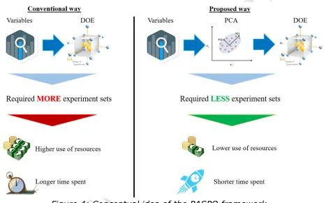
to include these parameters in the optimisation model. To address this issue, the PASPO framework which integrates PCA and DoE methodologies is proposed. The conceptual idea of this hybrid framework is illustrated in Figure 4. Initially, PCA is conducted to prioritise the variables based on their respective contribution scores. Only those (variables) with high contribution score are considered in DoE methodology. With the aid of the PCA methodology, the required number of experimental runs is expected to be reduced. This further lead to lower use of experimental resources (e.g., raw material) and time spent (e.g., working hours). Hence, the overall cost (material cost, energy cost, operator wages, etc.) is gradually reduced.

Figure 4: Conceptual idea of the PASPO framework

3.3.1 Principal Component Analysis (PCA)

M

A

NUS

C

R

IP

T

A

C

C

E

P

TE

D

instead of the covariance method (How and Lam, 2018b). The equation to evaluate the correlation between variables (Al-Sayed, 2015) is shown in Eq.(1) below.

( , ) = ∑ ̅ ̅ ( 1 )

In Eq.(1), and are the comparative variables; ̅ and ̅ are the average values of the corresponding variables; while and are the standard deviations of the corresponding variables, and n is the number of variable sets. The PC is evaluated from the correlational matrix, A, by solving an eigenvector-eigenvalue problem, as shown in Eq.(2). The first PC (or PC1) is responsible for the majority of variance in the data, followed by second PC (PC2) and so forth.

= ( 2 )

Where A refers to the correlation matrix, v refers to the eigenvector representing the regression coefficient of the principal components, while

λ refers to the eigenvalue which represents process variance (Shlens, 2014). Since the variables are multivariate and direct compiling the variables into the matrix will result in a less accurate model due to weight disproportion. A normalisation of process variables is required as shown in Eq.(3) below.

!"#$%& ₌ ̅ _{( 3 )}

To determine the numbers of PC included, the scree plot method with a heuristic minimum cumulative variance of 90% is used (Jackson, 1993). This is to ensure that the captured information is significant and data loss is acceptable (Rea and Rea, 2016).

'(). +, - ≥ 90 % ( 4 )

Next, the dimensions the multi-variable process inputs can be expressed as PC and be assessed using a scoring method (How and Lam, 2018b). The equation is shown in Eq. (5), where X refers to the normalised process variable matrix.

2' 3 4 = 5 ( 5 )

M

A

NUS

C

R

IP

T

A

C

C

E

P

TE

D

' 67 89(78 6 3 4:,$ =_{∑ ;%};%_<<,=_<,=;_; ∀9 ∈ @, ∀A ∈ B ( 6 )

To select critical variables as a representation of the full information, the contribution scores for each variable are sorted from large contribution to low contribution to plot a second scree plot. The cumulative contribution score is used as an indication for consideration of process variables for optimisation.

3.3.2 Design of Experiment (DoE)

The statistical significant process variables obtained from PCA in Section 3.3.1 are the input variables for the experiments, also known as factors, whereas the results from the experiments are recognised as responses. Subsequently, the predictive model is generated based on the changes in factors and responses from the experiments by regression analysis (Fisher, 1935). Response surface methodology (RSM) is used to generate multiple surface response plots which are used for the latter optimisation. A full factorial methodology is adopted for this framework, as the model includes complete information on the process data (Collins et al., 2009) for optimisation. Due to the inherent nature of process systems being highly complex (McKay et al., 1997), this work considers up to 4th order of interaction factor. Subsequently, an automatic selection algorithm with p-value as the criterion is used to remove terms that are detrimental (Anderson, 2018).

The multi-objective optimisation technique used is a two-step optimisation coupled with the desirability function. The desirability function approach is to convert each surface response into a desirability score di with a range of 0 to 1 (Derringer and Suich, 1980). The overall

desirability can be expressed as the following, where m is the total number of responses.

C = (D DE⋯ D ) / ( 7 )

The individual desirability function for a response, y with a maximum requirement is shown in Eq. (8) below.

D = H

0 I < K LM N_{O N}P K ≤ I ≤ R

1 I > R

( 8 )

M

A

NUS

C

R

IP

T

A

C

C

E

P

TE

D

D = H

1 I < K LU M_{U O}P K ≤ I ≤ R

0 I > R

( 9 )

For the above equations, L and U are the lower and upper limits respectively; r is the weight of the response. Setting r>1 prioritises the corresponding response while choosing 0<r<1 makes the response less important. Commonly, r is set to be one of the five standard levels as shown in Table 6 below (Kraber, 2009).

Table 6: Importance level and r value of desirability function Importance

Level

1 2 3 4 5

Pulses + ++ +++ ++++ +++++

r value 10-1 10-0.5 100 100.5 101

In this work, the importance level of each objective is prescribed by managerial decisions after evaluating market economics and product requirements. The pulses for importance level are presented in Table 7.

Table 7: Pulses for the importance of objectives

Properties SPE Product WFE Product

Yield +++++ +++

Quality +++ +++

Based on processing requirements, product yield is drastically more important than quality. Hence, a two-step optimisation method is applied to the desirability function for yield and quality sequentially as shown below.

374V 1: X, CM#%"& Y. 7. K- ≤ IZ[!"#\M, - ≤ R- ∀] ∈ ^ ( 10 )

374V 2: X, CZ[!"#\M Y. 7. K` ≤ IM#%"&, ` ≤ R` ∀a ∈ b ( 11 )

In addition, factors should be manipulated within minima and maxima boundary conditions based on equipment capacities and safety limits for the desired responses. Lastly, product quality is compared before and after DoE is performed.

3.4 Process Cycle Assessment

M

A

NUS

C

R

IP

T

A

C

C

E

P

TE

D

Process Cycle Assessment evaluates the process based on impact categories which are considered in LCA (WBCSD Chemicals, 2013). They include global warming potential (GWP) and acidification potential (AP), which are evaluated by the following equation:

cd2 = ∑f\ %! X_{% #ee# ,`}

`g ∑l m % \-g `,- hijk,- (12)

2 = ∑f\ %! `g X% #ee# ,`∑l m % \-g `,- hnk,- (13)

The assessment mainly considers mass flowrate of emission stream which is denoted by X_{% #ee# ,`</sub> for stream j. Mass fraction of contaminant component k in stream j is expressed as <sub>`,-} , while the specific potential environmental impact is expressed as h. Moreover, statistical process optimisation only considers the operating conditions of the process thus, Process Cycle Assessment only assesses the performance of the equipment and the final product.

4.0 Results

Large sets of processing data are collected from the Supervisory Control and Data Acquisition (SCADA) system of the oil re-refinery plant which enabled the effective use of principal component analysis and design of experiments. The validated process simulation model is also used to assist the design of experiments and for the case of 99% coverage score benchmark in Section 4.3. The following sections cover the detailed result of the principal component analysis, design and analysis of experiments, optimisation results of different coverage score and process cycle assessment.

4.1 Principal Component Analysis

M

A

NUS

C

R

IP

T

A

C

C

E

P

TE

D

Figure 5: Scree plot of principal component

M

A

NUS

C

R

IP

T

A

C

C

E

P

TE

D

Figure 6: Contribution of Process Variables on Principal Components

Having the critical PC decoupled into process variables, some highly significant peaks are observed to highly contribute to the processing system. Variables such as flash tank temperature, WFE temperature and level, SPE temperature and level were immediately identified to be significant in the process. These parameters that are identified decoupling the PC are highly logical, as temperature and levels within separators are variables that affect the separation efficiency and thermodynamics of the system. However, lesser significant variables are difficult to be studied in Figure 6, as the contribution of each variable has not been combined for direct comparison.

M

A

NUS

C

R

IP

T

A

C

C

E

P

TE

D

Figure 7: Prioritisation of process variables using contribution score

The factors that will be focused in DoE are operating temperature of the flash tank, WFE, SPE, operating pressure in WFE and SPE, operating level in WFE tank and SPE. These variables are selected based on a 95% coverage score and can be directly manipulated in the processing system. Furthermore, a study of 80% and 99% coverage score was carried out as a comparison. The 80% cumulative score case considers the temperature of WFE, SPE and flash tank, while 99% coverage score case considers all variables in 95% case with the addition of decanter level, decanter pressure and flash tank pressure.

4.2 Design and Analysis of Experiments

According to PCA result, factors considered for DoE includes operating temperature of flash tank (A), temperature of WFE (B), temperature of SPE (C), operating pressure of SPE (D), level of WFE (E) and level of SPE (F), while WFE (y1) and SPE (y2) product flow, WFE (y3) viscosity and SPE (y4) viscosity are the corresponding response in this study. The factorial design is used to generate desired responses. In addition, the design matrix is shown in Table 8, the “+” and “–” signs represent treatment combinations for the factors. As illustrated, there are seven degrees of freedom (DOF) for eight treatment combinations in which three DOF were associated with main effects of factor A, B, C, D and E.

Table 8: The design matrix for factorial design considering six factors

Run A B C D E F Labels

1 - - - 1

2 + - - - A

M

A

NUS

C

R

IP

T

A

C

C

E

P

TE

D

4 - - + - - - C

5 - - - + - - D

6 - - - - + - E

7 - - - + F

8 + + - - - - AB

9 + - + - - - AC

10 + - - + - - AD

11 + - - - + - AE

⁞ ⁞ ⁞ ⁞ ⁞ ⁞ ⁞ ⁞

53 - + + + + - BCDE

54 - + + + - + BCDF

55 - + + - + + BCEF

56 - + - + + + BDEF

57 - - + + + + CDEF

58 + + + + + - ABCDE

59 + + + + - + ABCDF

60 + + + - + + ABCEF

61 + + - + + + ABDEF

62 + - + + + + ACDEF

63 - + + + + + BCDEF

64 + + + + + + ABCDEF

Subsequently, factors and the responses were fitted with the regression model as shown in Eq.(14). Responses are denoted by yj, the regression

coefficient is indicated by βj whereby j can be any of the desired

responses projected by factors considered. Thus, each response will have a dedicated regression model.

The regression model for each response is used to generate a surface response plot as illustrated and explained below. The considered factors are up to 4th order interaction factors, then detrimental factors are removed using hierarchical automatic model selection algorithm with p-values as the criterion. All the considered possibilities of interaction factors considered to give an optimal surface response for yj is shown in the equation below.

I` = op,`+ onr + osr@ + otr' + ourC + ovrw + oxry + onsr @ + onlr ' +onur C + oslr@' + osur@C+ olur'C + olvr'w + olxr'y + ouvrCw + ouxrCy + ovxrwy + onslr @' + onsur @C + onlur 'C+ oslur@'C + oluvr'Cw + oluxr'Cy+ olvxr'wy + ouvxrCwy + onslur @'C

( 14 )

M

A

NUS

C

R

IP

T

A

C

C

E

P

TE

D

I = 22.601 − 1.003 + 7.345@ + 0.339w + 0.348y + 0.210 @ + 0.339wy

( 15 )

The most significant effect on the WFE product flow is the WFE temperature (B), which has the largest coefficient of 7.34. An inversely proportional relation can be observed between flash tank temperature (A) and WFE product flow. This is highly possible from the perspectives of separation sciences, as a higher temperature at the flash tank will cause the oil fraction to evaporate into the vapour fraction, reducing the amount of WFE oil products. SPE temperature (C) and pressure (D) have minimal effects on the WFE product flow. This is not surprising since the operating conditions of a downstream separation unit should give minimal effects to the units beforehand. However, level in WFE (E) and SPE (F) contribute to giving a higher WFE product flow, demonstrating positive coefficients of 0.339 and 0.348 respectively. Significant interaction factors are the interaction factors between flash tank temperature, WFE temperature (AB) and WFE level and SPE level (EF). Technically, the contributing interaction factors represent temperatures and levels of consecutive processing units.

M

A

NUS

C

R

IP

T

A

C

C

E

P

TE

D

Figure 8: Experimental values for WFE flowrate (LPM) as a function of the values predicted by the fitted model

Figure 9: Response surface for WFE flowrate (LPM) as a function of WFE temperature (°C) and Flash tank temperature (°C)

Next, analysis of WFE product viscosity (cSt) in the assessment of experimental design ranged from 6.96 to 10.63 cSt is used and the response is fitted in the regression model as shown in eq. (16). (The detailed ANOVA analysis can be found in Appendix Table 18)

Factor Coding: Actual WFE Flow (LPM)

30.6579

13.9767

X1 = A: Flash Temp X2 = B: WFE Temp

Actual Factors C: SPE Temp = 280 D: SPE Pressure = 0.05065 E: SPE Level = 55 F: WFE Level = 55

190 196 202 208 214 220

140 145

150 155

160 10

15 20 25 30 35

W

F

E

F

lo

w

(

L

P

M

)

M

A

NUS

C

R

IP

T

A

C

C

E

P

TE

D

IE = 8.728 − 0.206 + 1.633@ − 0.0214w + 0.0493 @ ( 16 )

It shows that the relationship of WFE temperatures (B) is proportional to WFE product viscosity with a positive regression coefficient of 1.633. The viscosity of WFE (y2) is found to be inversely proportional to flash temperature (A) and WFE level (E) with a negative coefficient of -0.206 and -0.0214 respectively. A higher temperature in the flash tank causes viscous oil additives within the oil is broken down, giving slightly lower WFE oil viscosity. Besides, at a significantly high level of WFE, the separation efficiency of the evaporator is affected and hence, WFE viscosity decreases. The significant interaction factor is the factor of the flash tank and WFE temperature (AB), which is the temperature interaction of consecutive processing units. Similarly, the WFE flow response, the regression coefficients of the viscosity of the WFE product are not significantly affected by the later process unit (SPE).

In addition, Figure 10 shows that the regression model for WFE product viscosity is appropriate to explore the trend of this response. For validation and visualisation, a response surface is generated using the regression model and shown in Figure 11. From the plot, WFE product viscosity is validated to be dependent on both flash and WFE temperature with stronger dependency for the latter. As illustrated in Figure 11, the colour of the response surface is warmer at the axis of WFE temperature but less warm at the axis of the flash tank temperature.

M

A

NUS

C

R

IP

T

A

C

C

E

P

TE

D

Figure 11: Response surface for WFE product viscosity (cSt) as a function of WFE temperature (°C) and Flash tank temperature (°C)

Analysis of SPE product flow (LPM) in the assessment of experimental design ranged from 0 to 30.54 LPM is used and the response was fitted in the regression model with regression coefficients as shown in Eq. (17) below. (The detailed ANOVA analysis can be found in Appendix Table 19)

IE = 10.148 + 0.446 − 5.485@ + 11.329' − 8.541C − 0.456w + 0.666y − 4.535@' +

2.095@' + 2.095@C + 4.905'C + 1.383'y − 2.095Cw + 3.931Cy − 4.113@'C +

5.189'Cy ( 17 )

From Eq. (17), the regression coefficients show that SPE product flow is affected by all main effects of Flash tank, WFE and SPE operating conditions. This is logical, as SPE is the final unit in the process and the product flow will depend on upstream units. In addition, Figure 12shows that the regression model for SPE product flow as a function of flash, WFE, SPE operating condition is fitting to inspect the trend of this response. Thus, a response surface is generated using the regression model as shown in Figure 13. From Figure 13(a), the model predicted that a higher SPE temperature (C) and higher WFE temperature (B) will improve the SPE product flow. Figure 13(b) and (c) also shows that having lower pressure in SFE improves the product flow, while the WFE level gives a slight proportional relationship with product flow. Moreover, increasing the WFE level (E) and SPE temperature (C) simultaneously give high SPE product flowrate.

Factor Coding: Actual WFE Visc (cSt)

10.6343

6.95882

X1 = A: Flash Temp X2 = B: WFE Temp

Actual Factors C: SPE Temp = 280 D: SPE Pressure = 0.05065 E: SPE Level = 55 F: WFE Level = 55

190 196 202 208 214 220 140 145 150 155 160 6 7 8 9 10 11 W F E V is c ( c S t)

M

A

NUS

C

R

IP

T

A

C

C

E

P

TE

D

Figure 12: Experimental values for SPE product flow (LPM) against the values predicted

Figure 13 (a)

Factor Coding: Actual SPE Flow (LPM)

30.5359

0

X1 = B: WFE Temp X2 = C: SPE Temp

Actual Factors A: Flash Temp = 150 D: SPE Pressure = 0.05065 E: SPE Level = 55 F: WFE Level = 55

220 250

280 310

340

190 196

202 208

214 220 -10

0 10 20 30 40

S

P

E

F

lo

w

(

L

P

M

)

B: WFE Temp (°C)

M

A

NUS

C

R

IP

T

A

C

C

E

P

TE

D

Figure 13 (b)

Figure 13 (c)

Figure 13: Response surface for SPE product flow (LPM) as a function of:

(a) WFE temperature (°C) and SPE temperature (°C)

(b) SPE pressure (bar) and WFE temperature (°C)

Factor Coding: Actual SPE Flow (LPM)

30.5359

0

X1 = B: WFE Temp X2 = D: SPE Pressure

Actual Factors A: Flash Temp = 150 C: SPE Temp = 280 E: SPE Level = 55 F: WFE Level = 55

0.0013 0.0154 0.0295 0.0436 0.0577 0.0718 0.0859 0.1 190 196 202 208 214 220 -10 0 10 20 30 40 S P E F lo w ( L P M )

B: WFE Temp (°C)

D: SPE Pressure (bar)

Factor Coding: Actual SPE Flow (LPM)

30.5359

0

X1 = C: SPE Temp X2 = F: WFE Level

Actual Factors A: Flash Temp = 150 B: WFE Temp = 205 D: SPE Pressure = 0.05065 E: SPE Level = 55

50 52 54 56 58 60 220 250 280 310 340 -20 -10 0 10 20 30 40 S P E F lo w ( L P M )

C: SPE Temp (°C)

M

A

NUS

C

R

IP

T

A

C

C

E

P

TE

D

(c) SPE temperature (°C) and WFE level (%)

Analysis of SPE product viscosity (cSt) in the assessment of experimental design ranged from 8.5 to 43.8 cSt is used and the response is fitted in the regression model with regression coefficients listed in Eq. (18).(The detailed ANOVA analysis can be found in Appendix Table 20)

I• = 19.527 + 1.357@ + 10.134' − 8.257C + 4.714@' − 4.842@C + 1.961'C +

7.806'y + 9.512'Cy ( 18 )

From Eq. (18), the SPE product viscosity mainly depends on SPE pressure (D) and temperature (C), as well as the WFE temperature (B). Thus, a response surface is generated using the regression model as shown in Figure 14. Subsequently, SPE product viscosity is found to improve with the simultaneous increase of SPE temperature and of WFE temperature from Figure 14(a). A similar relation to the SPE flow is found with the SPE pressure and level from Figure 14(b), in which a lower SPE pressure and higher WFE temperature give better product viscosity. This shows that lowering pressure while maintaining a high temperature in both SPE and WFE can improve SPE separation quality and yield.

Figure 14(a)

Factor Coding: Actual SPE Visc (cSt)

43.7527

8.54609

X1 = B: WFE Temp X2 = C: SPE Temp

Actual Factors A: Flash Temp = 150 D: SPE Pressure = 0.05065 E: SPE Level = 55 F: WFE Level = 55

220 250 280 310 340 190 196 202 208 214 220 0 10 20 30 40 50 S P E V is c ( c S t)

M

A

NUS

C

R

IP

T

A

C

C

E

P

TE

D

Figure 14: Response surface for SPE product viscosity (cSt) as a function of:

(a) WFE temperature (°C) and SPE temperature (°C)

(b) WFE temperature (°C) and SPE pressure (bar)

From the surface responses, the optimal operating temperatures of the flash tank, WFE and SPE are successfully established. To aid the understanding of the optimal combination of operating conditions for flash, WFE and SPE, an operating condition solution graph is plotted as illustrated in Figure 15. In details, Figure15(a), (b), (c), (d), (e) and (f) represent factors, while Figure 15 (g), (h), (i) and (j) represent the responses. Moreover, the factors in Figure 15(a), (b) and (c) are varied between their respective minimum and maximum operating temperatures denoted by the vertical boundary based on the actual capabilities of processing equipment. Furthermore, the vertical boundaries in Figure 15(g) and (h) are the process limit for WFE and SPE product viscosity. Note that higher viscosity is preferred for products of WFE and SPE.

Factor Coding: Actual SPE Visc (cSt)

43.7527

8.54609

X1 = B: WFE Temp X2 = D: SPE Pressure

Actual Factors A: Flash Temp = 150 C: SPE Temp = 280 E: SPE Level = 55 F: WFE Level = 55

0.0013 0.0154 0.0295 0.0436 0.0577 0.0718 0.0859 0.1 190 196 202 208 214 220 0 10 20 30 40 50 S P E V is c ( c S t)

M

A

NUS

C

R

IP

T

A

C

C

E

P

TE

D

Figure 15: Optimisation solution diagram (a) Operating temperature of flash

tank

(f) Operating level of WFE

(b) Operating temperature of WFE (g) WFE product flow (LPM)

(c) Operating temperature of SPE (h) WFE product viscosity (cSt)

(d) Operating pressure of SPE (i) SPE product flow (LPM)

(e) Operating level of SPE (j) SPE product viscosity (cSt)

Finally, comparisons between the factors and responses before and after statistical optimisation are shown in Table 9. Tremendous improvements are clearly seen in SPE product for its throughput (flow) at 84.4% and quality (viscosity) at 46.5%. This is achieved by lowering operating temperatures of the flash tank as much as 28.2% and 5.8% for WFE but an increase of 45.2% for SPE. The pressure in SPE remains unchanged while the level in the WFE and SPE increased by 9.1% and 20% respectively (two-tailed t-test can be found in Appendix Table 22).

Table 9: Comparisons between the factors and responses prior to and after optimisation

Process parameters Units Before After Change (%)

Flash Tank Temperature (°C) 222.6 159.86 28.2 WFE Temperature (°C) 228 214.73 5.8

SPE Temperature (°C) 231 335.5 45.2 SPE Pressure (bar) 0.0013 0.0013 0.0

WFE Level (%) 55 50.0 9.1

SPE Level (%) 50 60 20.0

WFE Product Flow (LPM) 20.75 26.16 26.1 WFE Product Viscosity (cSt) 10.56 10.0 5.3

M

A

NUS

C

R

IP

T

A

C

C

E

P

TE

D

4.3 Optimisation Results of Different Coverage Scores

Different coverage scores from the PCA model is used for DoE optimisation. Coverage scores of 80%, 95% and 99% (100% coverage score requires 49 DoE factors and resulting in 5.6x1014 number of runs) are used to benchmark the optimisation results. Each design will require an increase in DoE factors which, in return increases the number of runs. The optimised results are benchmarked in Table 10.

Table 10: Comparisons between the 80%, 95% and 99% coverage score (C.S.) optimisation

Variables Unit

80%

C.S.

(A)

Change (%)

95%

C.S.

(B)

Change (%)

99%

C.S.

(C) DoE

Factors - 3 - 6 - 17

Minimum Number

of Runs

- 8 - 64 - 262144

Coverage

Variance % 80 - 95 - 99

WFE Product

Flow

LPM 20.74 26.13 26.16 10.28 28.85

WFE Product Viscosity

cSt 10.00 0.00 10.00 0.00 10.00

SPE Product

Flow

LPM 23.66 19.53 28.28 2.58 29.01

SPE Product Viscosity

cSt 38.08 14.89 43.75 6.17 46.45

M

A

NUS

C

R

IP

T

A

C

C

E

P

TE

D

capital cost for 262080 extra experimental runs (4095 folds compared to Case B). Therefore, the 95% coverage score (Case B) used for this work is effective and efficient.

4.4 Process Cycle Assessment

The impact categories chosen to access environmental impacts for this case study are global warming potential (GWP) and acidification potential (AP). Standard indicators for GWP and AP which are carbon dioxide (CO2) and sulphur dioxide (SO2) equivalent are used respectively since it is common for oil products contaminated with hydrogen sulphide (H2S). Thus, characterisation models for conversion of natural and electricity to CO2 equivalent are shown in Table 11. Similarly, characterisation model for conversion of H2S to SO2 equivalent is shown in Table 12.

Table 11: Characterisation model for GWP (The Carbon Trust, 2011)

Energy

Natural gas

combustion Grid Electricity

Units kWh kWh

GWP (kgCO2-1) 5.3808 0.5246

Table 12: Characterisation model for AP (The Carbon Trust, 2011)

Acid Producer Hydrogen Sulphide (H2S)

Units kg

AP (kgSO2-1) 1.88

With the appropriate characterisation models, data for utilities, energy consumption and fractions of H2S in oil products are extracted from the simulation model and compared for both cases of before and after statistical process optimisation. Calculated results are shown in Table 13, Table 14and compared in Table 15.

Table 13: GWP for combustion of natural gas in furnace and electricity consumption for pump

Units

Furnace Pump

Before After %

Change Before After

% Change

Energy

(kWh) 93389.1 90139.6

3.54

763.9 757.3

86.6 GWP

(kgCO2-1) 17146.2 16549.6 400.7 397.3

M

A

NUS

C

R

IP

T

A

C

C

E

P

TE

D

Product

WFE SPE

Before After %

Change Before After

% Change

H2S (kg) 0.0057 0.0007

156.2

0.00 0.00

- AP (kgSO2-1) 0.01 0.00 0.00 0.00

Product

Lights Oil water

Before After %

Change Before After

% Change

H2S (kg) 62.11 4.80

171.3 1.02 0.95

7.1 AP (kgSO2-1) 116.76 9.03 1.92 1.78

Product

Asphalt

Before After %

Change

H2S (kg) 0.00 0.00

-

AP (kgSO2-1) 0.00 0.00

Table 15: Comparison of environmental performance for before and after statistical process optimisation

Impact category

GWP AP

Before After %

Change Before After

% Change

Value 17546.9 16946.9 3.42 118.7 10.8 90.89

M

A

NUS

C

R

IP

T

A

C

C

E

P

TE

D

threat. To conclude, the process achieved lean and green after statistical process optimisation.

5.0 Conclusion

In this work, a novel framework (PASPO) which integrates the use of process simulation, PCA, DoE and process cycle assessment is developed. The PASPO framework aims to provide a cost-effective and systematic way for process optimisation in the real chemical plant with the consideration of environmental impacts. Data from plant data historian are normally very big data sets that are difficult to be analysed. The significance of the PASPO framework is that it transforms plant operational data as the driving force for a practical and sensible plant-wide optimisation study. To elucidate the applicability and effectiveness of the PASPO framework, a real industrial case study of a waste oil re-refining plant (Pentas Flora Sdn. Bhd.) is carried out. This framework utilizes a novel correlational-based PCA implementation, in which processing variables are dimensionally reduced by both principal component’s cumulative variance and variable contribution score. After applying the PASPO framework, optimised operating conditions gave an increase in SPE product (main product) yield of 84.4% and WFE product improved by 26.1%. The quality of SPE also increased by 46.5%. In addition, results from DoE were assessed from the ecological point of view with process cycle assessment. The optimised processing conditions had improved Global Warming Potential (GWP) by 3.42% and Acidification Potential (AP) by 90.89%. With the aid of this framework, the waste oil re-refining plant can transform towards a leaner and greener operation. Evidently, emissions are reduced simultaneously with the enhancement of product throughput and quality. In all, the novel PASPO framework proposed has high potential in guiding engineers to design a sustainable process that considers the allowance for future expansions.

M

A

NUS

C

R

IP

T

A

C

C

E

P

TE

D

Acknowledgement

Research funding and support from Newton Fund and the EPSRC/RCUK (Grant Number: EP/PO18165/1) is gratefully acknowledged. Immense gratitude towards Pentas Flora Sdn. Bhd. for approving the case study to be carried out and performing lab test in their respected laboratory. Special thanks to Mr. Donny Goh and Ms. Tan Yuan Ni of Pentas Flora laboratory team.

Nomenclature

Abbreviation

WFE Wiped Film Evaporator

SPE Short Path Evaporator

DoE Design of Experiment

GWP Global Warming Potential

PCA Principal Component Analysis

H2S Hydrogen Sulphite

CO2 Carbon Dioxide

SO2 Sulphur Dioxide

LCA Life Cycle Analysis

LPM Liters Per Minute

GCMS Gas Chromatography–mass Spectrometry

AP Acidification Potential

GHG Greenhouse Gases

M

A

NUS

C

R

IP

T

A

C

C

E

P

TE

D

Appendix

The following is the paired t-test results for simulated and actual data. The results gave a p-value of 0.1384 (the difference is not statistically significant). The 95% confidence interval is from -8.6837 to 43.2157 with a mean of 17.2660.

Table 16: Paired t-test parameters (t=1.8473, dt=4, standard error of difference=9.346)

Group Simulated Data Actual Data

Mean 554.522 537.256

SD 483.6589 470.1995

SEM 216.2988 210.2796

N 5 5

The following are the regression coefficient and the statistical analysis of the design of experiment (DoE).

Table 17: Regression coefficients and ANOVA for the response of WFE product flow (LPM)

Source Coefficient Sum of

Squares

F-value p-value

(Prob>F)

Model - 16415.1560 116358.8793 <0.0001

Intercept 22.6013 - - -

A-Flash Temp

-1.0031 275.1277 11701.4628 <0.0001

B-WFE Temp

7.3449 11906.2998 506387.0382 <0.0001

E-SPE Level

0.3393 1.2691 53.9769 <0.0001

F-WFE Level

0.3483 0.6430 27.3466 <0.0001

AB 0.2099 5.7274 243.5931 <0.0001

EF 0.3393 0.5066 21.5483 <0.0001

Residual - 12.5085 - -

Cor Total - 16765.5081 - -

M

A

NUS

C

R

IP

T

A

C

C

E

P

TE

D

Table 18: Regression coefficients and ANOVA for response of WFE product viscosity (cSt)

Source Coefficient Sum of

Squares

F-value p-value

(Prob>F)

Model - 786.9929 165126.4812 <0.0001

Intercept 8.7278 - - -

A-Flash Temp

0.2055 12.4209 10424.5553 <0.0001

B-WFE Temp

1.6331 638.0008 535460.1176 <0.0001

E-SPE Level

-0.0214 0.0108 9.0462 0.0028

AB 0.0493 0.3514 294.9067 <0.0001

Residual - 0.6363 - -

Cor Total - 812.9685 - -

A-Flash temperature; B-WFE Temperature; C-SPE Temperature; D-SPE Pressure; E-SPE Level; F- WFE Level

Table 19: Regression coefficients and ANOVA for the response of SPE product flow (LPM)

Source Coefficient Sum of

Squares

F-value p-value

(Prob>F)

Model - 52398.7500 236.2309 <0.0001

Intercept 10.1482 - - -

A-Flash Temp

0.4463 60.5451 3.8214 0.0300

B-WFE Temp

-5.4853 6667.8276 420.8508 <0.0001

C-SPE Temp

11.3287 23774.3998 1500.5601 <0.0001

D-SPE Pressure

-8.5408 11734.2456 740.6261 <0.0001

E-SPE Level

-0.4555 12.4843 5.1568 0.0492

F-WFE Level

0.6656 13.2176 7.2031 0.0452

BC -4.5353 1975.1285 124.6635 <0.0001

BD 2.0954 367.1878 23.1757 <0.0001

CD 4.9047 1647.7490 104.0004 <0.0001

CF 1.3832 17.2610 10.4583 0.0499

DE -2.0946 26.1982 6.6535 0.0199

DF 3.9307 53.9186 3.4032 0.0456

BCD -4.1132 604.7040 38.1669 <0.0001

CDF 5.1890 53.5888 3.3823 0.0365

M

A

NUS

C

R

IP

T

A

C

C

E

P

TE

D

Cor Total - 60782.8346 - -

A-Flash temperature; B-WFE Temperature; C-SPE Temperature; D-SPE Pressure; E-SPE Level; F- WFE Level

Table 20: Regression coefficients for the response of SPE product viscosity (cSt) as a function of flash, WFE and SPE temperature (°C)

Factor Coefficient Sum of

Squares

F-value p-value

(Prob>F)

Model - 39819.2607 208.1621 <0.0001

Intercept 19.5272 - - -

B-WFE Temp

1.3569 472.7502 19.7711 <0.0001

C-SPE Temp

10.1338 19782.9625 827.3510 <0.0001

D-SPE Pressure

-8.2566 11825.1727 494.5452 <0.0001

BC 4.7141 2531.0360 105.8514 <0.0001

BD -4.8424 2220.4271 92.8614 <0.0001

CD 1.9611 270.6337 11.3183 0.0008

CF 7.8064 308.4422 12.8995 0.0004

CDF 9.5120 272.2222 11.3847 0.0008

Residual - 12672.9401 - -

Cor Total - 52630.4007 - -

A-Flash temperature; B-WFE Temperature; C-SPE Temperature; D-SPE Pressure; E-SPE Level; F- WFE Level

Table 21: Model regression parameters Model Properties WFE Viscosity Model SPE Viscosity Model SPE Flow Model WFE Flow Model

R2 0.9992 0.9586 0.9632 0.9992

Adj R2 0.9992 0.9549 0.9596 0.9992

Pred R2 0.9992 0.9446 0.9478 0.9992

Table 22: Confidence interval of optimised solution (Two-tailed t-test with n=1) Response WFE Viscosity (cSt) SPE Viscosity (cSt) SPE Flowrate (LPM) WFE Flowrate (LPM) Predicted Mean

10.0000 43.7527 28.2843 26.1653

M

A

NUS

C

R

IP

T

A

C

C

E

P

TE

D

Median

Std Dev 0.0345 4.8899 3.9804 0.1533

n 1 1 1 1

SE Pred 0.0361 5.9735 5.9261 0.1899

95% PI low 9.9290 32.0180 16.6424 25.7923

95% PI high 10.0710 55.4874 39.9262 26.5384

Table 23: Confirmation of optimisation results by sampling and error analysis

Properties WFE

Viscosity (cSt)

SPE Viscosity

(cSt)

SPE Flowrate

(LPM)

WFE Flowrate

(LPM) Optimised

Value

10.00 43.75 28.28 26.16

Sample 1 10.19 44.71 28.25 26.31

Sample 2 10.29 43.92 28.39 26.33

Sample 3 10.04 44.39 28.34 26.67

Signal 0.173333 0.59 0.046667 0.28

Pooled S.D. 0.088976 0.28098 0.050166 0.14089

Noise 0.072648 0.22942 0.040961 0.115036

T-value 2.385924 2.571708 1.139304 2.434016

P value (Type I Error)

0.075501 0.061867 0.318172 0.07167

P value (Type II Error)

M

A

NUS

C

R

IP

T

A

C

C

E

P

TE

D

References

Abdi, H. and Williams, L. J. (2010). Principal Component Analysis. John

Wiley &Sons, Inc.,2, 433-459.

Aida, S., Matsuno, T., Hasegawa, T., Tsuji, K. (2017). Application of principal component analysis for improvement of X-ray fluorescence images obtained by polycapillary-based micro-XRF technique. Nuclear

Instruments and Methods inPhysics Research B, 402, 267-273.

Al-Sayed, A. (2015). Principal component analysis within nuclear structure. Nuclear Physics A, 933, 154-164.

Alsayigh, A. (2015), Applying Lean Principles to Transform Conventional Oil & Gas

Amminudin, K., Enezi, T., Jubran, M., Hajji, A.,Bedoukhi, Z. (2011). Gas plant improves C3 recovery with Lean Six Sigma approach. 19th Annual Technical Conference of the GCC Chapter of the Gas Processors

Association.

Anderson, M. (2018). Design Expert Documentation. [online] Statease. Available at: https://www.statease.com/docs/v11/tutorials/combined-mix-process.html [Accessed 29 Oct. 2018].

Aspen Process Engineering Webinar (2006). Aspen HYSYS Property Packages Overview and Best Practices for Optimum Simulations. Aspentech, Galaxis, Singapore.

Atanas, J., Rodrigues, C., Simmons, R. (2016). Lean Six Sigma Applications in Oil and Gas Industry: Case Studies. International Journal

of Scientific and Research Publications, 6(5), 540-544.

Bhattacharya, A., Jain, R., Choudhary, A. (2011). Green Manufacturing

Energy, Products and Processes. The Boston Consulting Group, 1-24.

Box, G. E. P., Behnken, D. W. (1960). Some New Three Level Designs for the Study of Quantitative Variables. Technometrics, 2(4), 455-475.

M

A

NUS

C

R

IP

T

A

C

C

E

P

TE

D

Ning, C. and You, F. (2018). Data-driven decision making under uncertainty integrating robust optimization with principal component analysis and kernel smoothing methods. Computers and Chemical

Engineering, Volume 112, 190-210.

Collins, L., Dziak, J., Li, R. (2009). Design of experiments with multiple independent variables: A resource management perspective on complete and reduced factorial designs. Psychological Methods, 14(3), 202-224.

Čuček, L., Klemeš, J.,Kravanja, Z. (2012). A Review of Footprint analysis tools for monitoring impacts on sustainability. Journal of

Cleaner Production, 34, 9-20.

Chiang, L., Lu, B., Castillo, I. (2017). Big data analytics in chemical engineering. Annual review of chemical and biomolecular engineering, 8, 63-85.

Derringer, G. and Suich, R. (1980). Simultaneous Optimization of Several Response Variables.Journal of Quality Technology, 12(4), 214-219.

Drovandi, C.C., Holmes, C., McGree, J.M., Mengersen, K., Richardson, S., Ryan, E.G. (2017). Principles of experimental design for Big Data analysis. Statistical science: a review journal of the Institute of

Mathematical Statistics, 32(3), p.385.

Fisher, R. A. (1935). The Design of Experiments. Edinburg: Oliver & Boyd. Gunst, R. F. and Mason, R. L. (2009). Fractional factorial design. WIREs

CompStat,1, 234-244.

Halvorsen, M., Elseth, G.,Naevdal, O. (2012). Increased oil production at Troll by autonomous inflow control with RCP valves. SPE Annual Technical Conference and Exhibition.

Hostelling, H. (1933). Analysis of a complex of statistical variables into principal components. Journal of Educational Psychology, 24(6), 417-441.

How, B.S. and Lam, H.S. (2018a). Sustainability evaluation for biomass supply chain synthesis: Novel principal component analysis (PCA) aided optimisation approach. Journal of Cleaner Production, 189, 941-961.

M

A

NUS

C

R

IP

T

A

C

C

E

P

TE

D

Process Integration and Optimization for Sustainability, doi.org/10.1007/s41660-018-0036-3.

Hu, Y., Li, G., Chen, H., Li, H., Liu, J. (2016). Sensitivity analysis for PCA-based chiller sensor fault detection. International Journal of Refrigeration, 63, 133-143.

Huda, L. and Matondang, R. (2018). The lean ergonomics in green design of crude palm oil plant. IOP Conference Series: Materials Science and

Engineering, 309, 012109.

International Organization for Standardization (ISO) (2006). ISO 14044 :Environmental management - Life cycle assessment - Requirements and

guidelines. 1st ed. Geneva: ISO.

Jackson, D. (1993). Stopping Rules in Principal Components Analysis: A Comparison of Heuristical and Statistical Approaches.Ecology, 74(8), pp.2204-2214.

Jolliffe, I. and Cadima, J. (2016). Principal component analysis: a review and recent developments. Philosophical Transactions of the Royal Society

A: Mathematical, Physical and Engineering Sciences, 374(2065),

20150202.

Joly, M., Moro, L., Pinto, J. (2002). Planning and scheduling for petroleum refineries using mathematical programming. Brazilian Journal of Chemical Engineering, 19(2), 207-228.

Klemeš, J. and Kravanja, Z. (2013). Forty years of Heat Integration: Pinch Analysis (PA) and Mathematical Programming (MP). Current Opinion

in Chemical Engineering, 2(4), 461-474.

Klemeš, J., Varbanov, P.,Huisingh, D. (2012). Recent cleaner production advances in process monitoring and optimisation. Journal

of Cleaner Production, 34, 1-8.

Klemeš, J., Dhole, V., Raissi, K., Perry, S.,Puigjaner, L. (1997). Targeting and design methodology for reduction of fuel, power and CO2 on total sites. Applied Thermal Engineering, 17(8-10), 993-1003.

Kraber, S. (2009). Response Surface Optimization. Stat-Ease Inc.

M

A

NUS

C

R

IP

T

A

C

C

E

P

TE

D

Lam, H., How, B. and Hong, B. (2015). Green supply chain toward sustainable industry development. Assessing and Measuring

Environmental Impact and Sustainability, 409-449.

Leong. W.D., Lam. H.L., Ng. W.P.Q., Lim. C.H., Tan. C.P., Ponnabalam. S.G., (2018), Lean and Green Manufacturing - A Review on Application and Effect. Process Integration and Optimization for Sustainability. (In Press)

McKay, B., Willis, M., Barton, G. (1997). Steady-state modelling of chemical process systems using genetic programming. Computers &

Chemical Engineering, 21(9), 981-996.

Morita, T., Yogo, S., Koike, M., Hamaguchi, T., Jung, S., Koshijima, I., Hashimoto, Y., (2013). Detection of cyber-attacks with zone dividing and PCA. Procedia Computer Science, 22, 727-736.

Murray, P. and Forfar, L. (2017). The Application of Advanced Design of Experiments for the Efficient Development of Chemical Processes.

Chemical Informatics, 03(02).

Nobi, A., Alam, S., Lee, J.W., (2017). Dynamic of consumer groups and response of commodity markets by principal component analysis. Physica A: Statistical Mechanics and its Applications, 482, 337-344.

Pearson, K. (1901). On lines and planes of closest fit to systems of points in space. Philosophical Magazine,2,559-572. http://pbil.univ-lyon1.fr/R/pearson1901.pdf

Porter, M. E. and Linde, V. D. (1995). Green and competitive: Ending the stalemate. Harvard Bus. Rev., 73(5), 120-134.

Production Operations in a Gulf State into Cleaner Energy, PhD Thesis, Loughborough University, England.

Rea, A. and Rea, W., (2016). How Many Components should be Retained from a Multivariate Time Series PCA? arXiv preprint arXiv:1610.03588.

Schneider, D. F. (1997). Debottlenecking Options and Optimization,

Houston: Stratus Engineering, Inc.

Shlens, J. (2014). A Tutorial on Principal Component Analysis.

M

A

NUS

C

R

IP

T

A

C

C

E

P

TE

D

Smith, R. and Linnhoff, B. (1988). Design of separators in the context of overall processes. Chemical Engineering Research and Design, 66(3), 195-228.

Telford, J. K. (2007). A brief introduction to design of experiments.

JohnsHopkins APL Technical Digest (Applied Physics Labor