Stabilizing l1-norm prediction models by supervised feature grouping

(1)

Stabilizing

l

1

-norm prediction models by supervised feature grouping

Iman Kamkar

⇑

, Sunil Kumar Gupta, Dinh Phung, Svetha Venkatesh

Centre for Pattern Recognition and Data Analytics, Deakin University, Australia

a r t i c l e i n f o

Article history:

Received 14 May 2015 Revised 18 November 2015 Accepted 23 November 2015 Available online 9 December 2015

Keywords:

Supervised feature grouping Feature selection

Stability Lasso

a b s t r a c t

Emerging Electronic Medical Records (EMRs) have reformed the modern healthcare. These records have great potential to be used for building clinical prediction models. However, a problem in using them is their high dimensionality. Since a lot of information may not be relevant for prediction, the underlying complexity of the prediction models may not be high. A popular way to deal with this problem is to

employ feature selection. Lasso andl1-norm based feature selection methods have shown promising

results. But, in presence of correlated features, these methods select features that change considerably with small changes in data. This prevents clinicians to obtain a stable feature set, which is crucial for clin-ical decision making. Grouping correlated variables together can improve the stability of feature selec-tion, however, such grouping is usually not known and needs to be estimated for optimal performance. Addressing this problem, we propose a new model that can simultaneously learn the grouping ofcorrelated features and perform stable feature selection. We formulate the model as a con-strained optimization problem and provide an efficient solution with guaranteed convergence. Our experiments with both synthetic and real-world datasets show that the proposed model is significantly more stable than Lasso and many existing state-of-the-art shrinkage and classification methods. We fur-ther show that in terms of prediction performance, the proposed method consistently outperforms Lasso and other baselines. Our model can be used for selecting stable risk factors for a variety of healthcare problems, so it can assist clinicians toward accurate decision making.

1. Introduction

Nowadays, healthcare data such as medications, pathological results and radiological images are being recorded digitally in form of Electronic Medical Records (EMRs). EMR data have good poten-tial to be used for clinical research and decision making [1]. Although this data consist of rich information about patients, con-siderable amount of it is irrelevant and redundant for prediction. Therefore, to build accurate prediction models from such a high-dimensional data, feature selection is essential.

A great variety of feature selection methods have been pro-posed and proved to be effective in improving prediction accuracy. Nevertheless, a relatively neglected issue in these methods is their ability to select stable features, which remains an unresolved prob-lem[2]. The stability of a feature selection algorithm is its robust-ness to slight changes in data and is defined as the degree of agreement over feature sets selected by an algorithm when trained

on slightly different training sets. Stability is particularly important for knowledge discovery problems, where features carry intuitive meanings and actions are taken based on these features. This is indeed the case in healthcare with applications such as identifying risk factors for cancer survival or hospital readmission. In all of these applications, selected features must be stable to help clini-cians towards accurate and consistent decision making.

The main reason of feature instability is existence of highly cor-related features in dataset[3]. This scenario is often encountered when data is high dimensional[4,5]. In this context, many feature selection algorithms would discard features that are correlated to selected features but still associated with response. In knowledge discovery problems, such feature selection methods would miss on important knowledge about correlated features that are dis-carded. Further, as a result of discarding correlated features, from each set of correlated features, feature selection algorithms tend to selectdifferentfeatures when trained on slightly different train-ing sets[2]. The other reason of instability is feature selection algo-rithm design [3]. Mostly, the main goal of feature selection algorithms is to select the minimum subset of the features that results in a prediction model with thebestpredictive performance. This goal may not be necessarily aligned with feature stability[2,6]. http://dx.doi.org/10.1016/j.jbi.2015.11.012

E-mail addresses:[email protected](I. Kamkar),[email protected]. au(S.K. Gupta),[email protected](D. Phung),svetha.venkatesh@deakin. edu.au(S. Venkatesh).

Contents lists available atScienceDirect

Journal of Biomedical Informatics

(2)

Among many feature selection methods that have been intro-duced in literature, penalized regression methods such as Lasso that usel1-norm penalty to encourage sparsity have been shown to be effective[7]. Although Lasso has achieved great success in many applications[8–10], it showsunstablebehavior in presence of groups of highly correlated features[11,12]. The Lasso’s instabil-ity in selecting features is due to its tendency to select randomly one feature from a group of correlated features. Small changes in data result in a significant change in selected features leading to unstable models. A graphical illustration of this instability is shown inFig. 1.

The previous work on stabilizing l1-norm methods has exploited domain knowledge to find groups of correlated features and attempted to select most of the correlated features. For exam-ple, when features have an intrinsic hierarchical structure, tree-Lasso has been used as a method to improve feature selection sta-bility[13,14]. Similarly, when features have an ordering and corre-lation of features is mainly due to their ordering, fused Lasso[15] can be used to select neighboring features and thus improve fea-ture stability. However, in most of the feafea-ture selection applica-tions, such a structure is not present and these methods may not be applicable. Limited work has been done to address the feature stability problem in a general context. Oscar[16]is a recent feature selection method that aims to improve feature stability by group-ing correlated features and assigngroup-ing equal weights to them. How-ever, in real-world applications, many features are only partially correlated, meaning that Oscar either does not group them together or if grouped together makes their weights equal, which may cause degradations in prediction performance[17]. Thus the problem of stable feature selection remainsopen.

Addressing this gap, we propose a framework to improve the stability of Lasso by grouping correlated features and selecting informative groups instead of each individual feature. Feature grouping is learned within the model using supervised data and therefore is aligned with prediction goal. To this end, we learn a matrixG, where each column ofGrepresents a group such that if a featurepbelongs to a groupkthenGik¼1, otherwise 0. Since learning a binary matrixGrequires integer programming and is computationally expensive, we relax G to be non-negative. An added advantage of using non-negativity is that each column of G now contains real-valued non-negative values, which can be interpreted as weight/importance of a feature in the group. We also impose orthogonality constraint onGto ensure that a feature is part of only one group. The proposed model is formulated as a constrained optimization problem combining both feature group-ing and feature selection in a sgroup-ingle step. To solve this problem, we propose an efficient iterative algorithm with theoretical guar-antees for its convergence. We demonstrate the usefulness of the model via experiments on both synthetic and real datasets. We compare our model with several other baseline models demon-strating its superiority for both feature stability and prediction performance.

In summary, our main contributions are:

Proposal of a new model aimed to achieve stable feature selec-tion in general context. The proposed model improves the sta-bility of Lasso by grouping correlated features and selecting informative groups instead of each individual feature.

Formulation of the model using a constrained optimization problem and providing an iterative solution with guaranteed convergence.

Comparison of the stability of the proposed model with baseline regression and feature selection methods such as Ridge, Lasso, Elastic net, K-means+Lasso, K-means+GroupLasso and Oscar, showing that its stability is significantly better than Lasso and comparable with other methods.

An extensive experimental study that shows the predictive per-formance of the model is consistently better than those of base-line methods.

Our model can be applied for selecting stable risk factors in healthcare domain and has potential to assist clinicians toward accurate decision making. Going beyond, our model can be used in any real-world application where stability of features is impor-tant such as biomarker discovery in genomics and proteomics applications.

2. Related works

Existing methods which are developed for stable feature selection can be categorized into three classes based on the way they manage different sources of instability[3]. (1) Ensem-ble feature selection methods that consider stability in the stage of algorithm design. (2) Sample injection methods that try to address the issue of small sample size in high dimensional prob-lems by increasing the sample size. (3) Group feature selection methods that consider feature grouping to increase stability of the feature selection method. In this section, we briefly discuss these methods.

2.1. Ensemble feature selection methods

Generally, ensemble learning methods such as bagging[18]and boosting[19]are widely used in statistics and machine learning. These methods combine multiple feature selection models to obtain better results than could be obtained from any single model. Ensemble feature selection methods use the following two steps in their procedure:

They create different feature selectors.

They aggregate the results of constituent feature selectors and generate the ensemble output.

The second step in this procedure can be modeled as a rank aggregation problem that combines multiple rankings into a con-sensus ranking[20,21]. In[22]authors show that one of the essen-tial steps in building a successful ensemble learner is generating a set of diverse components learners. To this end, two strategies are used:

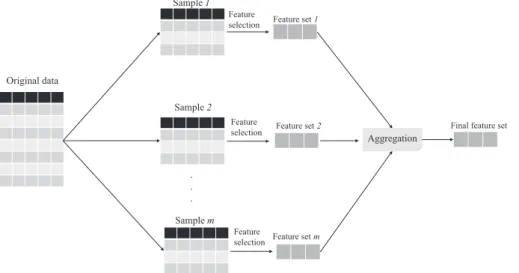
1. Ensemble feature selection methods that run a feature selection algorithm with different sub-samples. In these methods differ-ent sub-samples are generated from original data. Then these sub-samples are used by a feature selection algorithm to select the most informative features and finally a consensus output is built using a rank aggregation method. This process is shown in Fig. 2. The methods proposed in[23–26]are classified into this category.

2. Ensemble feature selection methods that use different feature selection algorithms as their component learners. These meth-ods are different from previous methmeth-ods in two ways: Firstly, they use different feature selection algorithms instead of one, and secondly, they perform local feature selection on the origi-nal data without sampling. Methods developed in[27–30]fall in this category.

2.2. Feature selection with sample injection

In some applications such as bioinformatics, there are small number of samples in high dimensional data, causing instability in feature selection. One way to overcome this problem, is

(3)

increasing number of samples. Nevertheless, obtaining new sam-ples is often costly and time consuming. Under these constraints, two alternative methods are used: (1) Using test data to increase the sample size in feature selection, which can be formulated as a transductive learning problem[31–33], and (2) Using artificial training samples generated from distribution of original training data. The artificial samples are augmented with original samples in training process[34].

2.3. Group feature selection

In high dimensional data, it is common to find groups of corre-lated features. Often these groups are consistent to the variation of training data. Therefore, group feature selection can be used as a solution to increase stability of feature selection algorithms. These groups can be identified by using prior domain knowledge (knowledge-driven) or may be learned from data (data-driven).

Knowledge-driven methods have mostly been used in the field of bioinformatics to find genes that have coherent expression pat-terns in the same gene set using large protein networks. The main idea here is to find a group of genes from the same pathway, which are associated with response and then convert this group into a new super feature for subsequent feature selection. Methods dis-cussed in[35–39]are some examples of knowledge-driven meth-ods that try to identify markers as gene sets instead of individual genes. These methods use different strategies for group generation and transforming groups into super features. In group generation procedure, we can use all the genes in a same pathway, or we

can search for a subset of genes to obtain a better discriminating group. To convert each group to a super feature, we can use differ-ent summary statistics methods such as mean or principle compo-nent analysis.

Data-driven group formation models identify feature groups using either cluster analysis[40–43]or density estimation[44,2]. Cluster analysis methods use clustering algorithms such as K -means to group correlated features, whereas density estimation methods tend to group correlated features using kernel density estimation.

There is another class of related works that aim to stabilizel1 -norm methods such as Lasso. For example, Group Lasso can be used as a remedy to stabilize Lasso when feature grouping information isavailable. This method performs feature selection at group level [11]. A modification of group Lasso that operates on overlapping groups is proposed in [45,46]. When features have an intrinsic hierarchical and tree structure, tree-Lasso can be used as a method for increasing feature selection stability [13,14]. When grouping information is not available, feature correlations may serve as an alternative. Elastic net is an example of this class, which reduces the randomness of Lasso by using a combination ofl1andl2 penal-ties[47]. However, the final model obtained using this combina-tion is less sparse and has longer list of features. When features are ordered and correlated, fused Lasso is a useful method that can exploit the structure of the features[15]. To group features, fused Lasso enforces the successive features in a local neighbor-hood to be similar. However, such an ordering on features does not exist in many applications rendering this method inapplicable.

G1 G2 G3 G4

Data matrix with groups

of correlated features

Selected features using Lasso

Fig. 1.Instability behavior of Lasso when selecting features in presence of correlated feature groups.

Original data Sample1 Sample 2 Samplem Feature selection Feature selection Feature selection Feature set 1 Feature set 2 Feature set m Aggregation

Final feature set

. . .

Fig. 2.Ensemble feature selection approach using sub-sampling of original data. First, different sub-samples of the original data are built and informative features of each sub-sample are obtained. Then the final feature set is selected using a rank aggregation method.

(4)

Grouping pursuit[48]is another method that tries to select all pos-sible groups, but it cannot achieve sparse model. Oscar [16] is another alternative that performs feature grouping and feature selection, simultaneously. By applying a combination of l1 and pairwisel1norm penalties, it imposes sparsity and equal feature

weight for highly correlated features. However, assigning equal weights to the features that are only partially correlated may degrade prediction performance of the model[17]. Furthermore, because of using l1 regularization term, any two variables that

are nearby or extremely far from each other, will be assigned the same penalty. This leads to unnecessary bias especially for large coefficients[49].

3. Feature stability

Stability of a feature selection algorithm is measured by consis-tency across various feature sets produced with slightly differing training sets, drawn from the same distribution [50,5]. In order to assess the stability of feature selection algorithms, different methods have been introduced. These methods can be categorized into three different groups[51]. First group, known asstability by index, considers the indices of the selected features. In this cate-gory, the selected features have no particular order or correspond-ing relevance weight. In the second group, known asstability by weight, degree of relevance of each feature is measured by a weight assigned to the feature. In the third group, which is calledstability by rank, the feature’s order is important in evaluation of stability. In this group, each feature is assigned a rank that shows its importance.

In other words, if a training set containspfeatures denoted by the vector f¼ ðf1;f2;. . .;fpÞ, then after using a feature selection algorithm we will have:

In case of stability by index, a subset of features: S¼ ðs1;s2;. . .;spÞ,si2 f0;1g, where 1 shows the presence of a feature and 0 shows its absence.

In case of stability by weight, a weighing:w¼ ðw1;w2;. . .;wpÞ, w#Rp_.

In case of stability by rank, a ranking: r¼ ðr1;r2;. . .;rpÞ, 16ri6p.

In order to assess the stability of a feature selection algorithm, we need a similarity measure for the above mentioned representa-tions. To measure similarity between subsets of features, we use Jaccard index – a metric that measures similarity between two sets. If there are two sets of featuresSqandSq0, the Jaccard index JðSq;Sq0Þis defined as JðSq;Sq0Þ ¼ Sq T Sq0 Sq S Sq0 : ð1Þ

To define a stability measure using Jaccard index, we generateQ sub-samples of the training data, indexed asq¼1;. . .;Q. For each sub-sample, we run feature selection model and obtain a feature set, denoted by Sq. Given feature setsS1;. . .;SQ,Jaccard stability measure(JSM) is defined as the average of Jaccard indices over each pair of feature sets, i.e.J S q;Sq0. Formally, we have

JSM¼ 2 QðQ1Þ X Q1 q¼1 XQ q0¼qþ1 J S q;Sq0: ð2Þ

The other stability measure in this category is Kuncheva Index [50]. As this metric focuses on topkselected features, we consider the following setting for it. We generate Q sub-samples of the training data and in each sub-sample we select top k features based on their importance. The importance of each feature is

calcu-lated as the product of the feature’s weight and its standard devi-ation in the training dataset [52]. Finally, the feature subsets S¼ fS1;. . .;SQgare obtained wherejSij ¼k. ConsideringSqandSq0 again as two feature sets, Kuncheva Index is defined as

ICðSq;Sq0Þ ¼ rpk 2

kðpkÞ; ð3Þ

wherejSqTSq0j ¼randpis the number of features. The Kuncheva Index is bound in½1;1. This metric tries to correct overlappings occurred by chance. In other words, for independently drawn fea-turesSq andSq0; I_CðS_q;S_q0Þassumes values close to zero becauser is expected to be aroundk2

n.

Taking the average of all pairs, the overall Kuncheva Index is computed as IS¼ 2 QðQ1Þ X Q1 q¼1 XQ q0_¼qþ1 ICðSq;Sq0Þ: ð4Þ

To measure similarity between two weightingsw; w0_obtained

from a feature selection algorithm, we use Pearson’s correlation coefficient: PCCðw;w0Þ ¼ P jðwj

l

wÞðw0j

l

w0Þ ffiffiffiffiffiffiffiffiffiffiffiffiffiffiffiffiffiffiffiffiffiffiffiffiffiffiffiffiffiffiffiffiffiffiffiffiffiffiffiffiffiffiffiffiffiffiffiffiffiffiffiffiffiffiffiffiffiffiffi P jðwj

l

wÞ 2P iðw0j

l

w0Þ2 q ; ð5Þ

where PCC2 ½1;1. A value of 1 means that weightings are per-fectly correlated, a value of 0 means that there is no correlation between weightings and a value of 1 means they are anticorrelated.

To measure rank based similarity between two rankingsr;r0_{, we}

use Spearman’s rank correlation coefficient: SRCCðr;r0Þ ¼16X

j

ðrjr0jÞ

pðp2_1Þ: ð6Þ

Similar to Pearson’s correlation, the possible range of values for SRCC is½1;1, where 1 shows that two rankings are identical, 0 shows that there is no correlation between two rankings and1 shows that rankings are in reverse order.

To estimate the stability of a feature selection algorithm for a given dataset, we generateQsub-samples of the training set and apply the feature selection algorithm to each sub-sample, where it results in a feature preference for each sub-sample. Using the appropriate similarity measure, we compute the similarity between each pair of feature preferences and finally the stability of the feature selection algorithms is obtained by averaging simi-larity over all pairs.

As feature selection algorithms may use different scales for assign weights to the feature weightings and PCC works directly on the obtained weight vectors, its results may not be directly comparable across different algorithms. Hence, to evaluate stabil-ity of each algorithm we only use SRCC, JSM and Kuncheva Index. Note that high value for SRCC implies that ranks of features do not vary a lot for different training sets and high value for JSM means that the selected features do not change significantly.

4. Methodology

4.1. Predictive grouping elastic net

In this section, we propose our framework that can simultane-ously group correlated variables and select the best group of vari-ables in a supervised manner. We consider a standard supervised learning setting with datafdi;yig

n

i¼1, wheredi2Rp is the feature vector representingpfeatures andyiis the target value (for regres-sion) or label (for classification). Collectively, we represent the data

(5)

using a matrixD2Rnp_{, where each row corresponds to the} _i_th instance; similarly we havey¼ ðy1;. . .;ynÞ

T

, a vector for target val-ues. We denote thejth column of the data matrixDbydj2Rn. We assume that the features have been standardized to have mean zero and anl2norm of 1; in other words:PiDij¼0,PiD

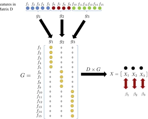
2 ij¼1. In presence of correlated features, our goal is to identify and group them. By doing this, not only the stability of feature selection can be improved[53], but also the estimator’s variance can be reduced[48]. This reduction of variance leads to better prediction performance. To this end, we learn a matrixG2RpK_{, where each} column ofGrepresents a feature grouping such that if feature p is part of group k, then we have Gpk¼1 and 0 otherwise. By restrictingGto be a binary matrix, the optimization procedure of our model would be an integer programming problem, which is NP-hard. Therefore, for simplicity in optimization process, we relax Gto be non-negative. Moreover, the non-negative values inGcan be interpreted as weight of each feature within each group and can be used to identify the importance of each feature in its group. InFig. 3, the procedure of grouping features and assigning weights to each group is shown graphically. As seen from the figure, the data matrixDhas unknown groups of highly correlated features. The proposed method can find these correlated groups and build the grouping matrix G. Multiplying Dby G obtains the ‘‘super-features” X2RnK ₍_K_<_p_{), which are the representatives of the} correlated features in each group. The proposed algorithm finds the coefficient vectorb2RK1, for super-features X. The weight vectorw2Rp1_{for each feature in matrix}_D_{can still be obtained} asw¼Gb.

Using the above feature grouping scheme, we formulate the fea-ture selection as an optimization problem with the following objective function: min b;GP0Jðb;GÞ ¼kyDGbk 2 2þk

Xð

bÞ þdtrðIG T GÞ; ð7Þ where

X

ðbÞ ¼ ð1

a

Þk kb 1þ

a

₂k kb 2 2;

a

2 ½0;1:

The first term inJðb;GÞensures model fitting;XðbÞis a regulariza-tion term that prevents overfitting, and the last term with regular-ization parameter d2 ð0;1Þ guarantees the orthogonality of the groups i.e. it ensures that each variable belongs only to one group. We call this modelpredictive grouping Elastic net(pg-EN).

4.1.1. Optimization algorithm

The cost function of pg-EN in(7)is convex forbandG individ-ually, but not for both. Therefore, we do not expect an optimization algorithm to find a global minimum. Thus, we minimize the cost function via an iterative algorithm that updates G and b

alternatively.

A step-by-step procedure for optimization of the proposed model is provided inAlgorithm 1. The first step in the optimization algorithm is initialization ofG. We can either randomly assign fea-tures to the groups or this can be done usingK-means algorithm. However, usingK-means results in faster convergence of the algo-rithm (observed empirically in our experiments). As the optimiza-tion procedure is iterative, in the second step we solve Eq.(7)with respect tobwhile fixingG. This leads to Eq.(8), which is identical to the Elastic net cost function and is solved using coordinate des-cent approach (see, for example,[54]). In the next step, we opti-mize Eq.(7)with respect toG, whenbis fixed. This results in Eq. (9). To solve this equation, we use the multiplication update rule, which is adapted from the semi-NMF model [55]. Thus, G is updated using

Algorithm 1. Algorithm for solving pg-EN optimization problem.

InitializeGas a solution of aK-means to cluster features. – ifdi2kthenGik¼1

– elseGik¼0 – endif

HoldGfixed and solve Eq.(7)forb. DefiningX¼DG, that is, solve arg min b JðbÞ ¼ 1 2kyXbk 2 2þkð1

a

Þk kb 1þk

a

2kbk 2 2: ð8Þ

Holdbfixed and solve Eq.(7)forG. If we defineA¼bbT, B¼DT_D_and_C_¼_DT_y

bthat is, solve

arg min G kyDGbk 2 2þdtrðIG T GÞ n o ð9Þ Gik Gik ffiffiffiffiffiffiffiffiffiffiffiffiffiffiffiffiffiffiffiffiffiffiffiffiffiffiffiffiffiffiffiffiffiffiffiffiffiffiffiffiffiffiffiffiffiffiffiffiffiffiffiffiffiffiffiffiffiffiffiffiffiffiffiffiffiffiffiffiffiffiffiffiffiffiffi BGAþ ikþ B þ_GA ikþC þ ikþdGik BþGAþ ikþ B _GA ð ÞikþC ik s ; ð10Þ

where the positive and negative parts of a matrixTare defined as Tþ_ik¼0:5ðjTikj þTikÞandTik¼0:5ðjTikj TikÞ. The details about the update rule forG(Eq.(10)), is provided in Section4.1.3.

4.1.2. Computational complexity

AsK<p, the computational complexity of pg-EN for Step 1, in presence ofKgroups, is much smaller compared to standard Lasso. Computational complexity for Step 2 is of the order mðK2þKp2þpK2þpnþpKÞ, wheremis the number of iterations of the algorithm. The empirical convergence of Algorithm 1 is shown inFig. 4for two of the real-world datasets used in the paper. As seen from the figure, the algorithm converges usually within 50–60 iterations.

4.1.3. Theoretical guarantees for convergence

In this section we prove the convergence of the cost function in Eq.(7)under the updates rule of(8) and (10). The non-negative constraint ofG, lets us to proceed along the lines of non-negative matrix factorization [56]and semi-nmf[55]to prove its conver-gence. However, the main difference here is that our model con-tains supervised information (y).

Theorem 1. (1) Fixing G; Jðb;GÞ is identical to Elastic net cost function and converges using coordinate descent or proximal gradient method. (2) Fixingb, the cost function Jðb;GÞ, decreases monotonically under the update rule of(10)for G.

Proof. To prove part 1, see[57]that discusses about the conver-gence properties of coordinate descent for convex problems or see [58] that discusses about the proximal gradient algorithms for solving convex optimization problems. To prove part 2, which is a constrained optimization problem we show two results: (a) We show that at convergence, the solution of the update rule of (10) satisfies the Karush–Kuhn–Tucker condition. This is presented in Proposition 1. (b) We show that the cost function Jðb;GÞconverges under the update rule of(10). This is shown in Proposition 2. h

Proposition 1. The limiting solution of the update rule in(10) satis-fies Karush–Kuhn–Tucker condition.

(6)

Proof. See the appendix.h

Proposition 2. The cost function J is non-increasing under the update rule(10).

Proposition 3. Based on the objective function JðHÞdefined in(.5) with nonnegative matrices, the following

ZðH;H0Þ ¼ X ik 2CþikH 0 ik 1þlog Hik H0ik þX ik 2Cik H2 ikþH 02 ik H0ik þX ik ðBþH0AþÞikH 2 ik H0ik X i;j;k;l BijH 0 jkA þ klH 0 il 1þlog HjkHil H0jkH 0 ik ! X i;j;k;l BþijH0jkA klH0il 1þlog HjkHil H0jkH 0 ik ! þX ik ðBH0AÞikH 2 ik H0ik X i;k dH0ik2 1þlog H2 ik H0ik2 ! ; ð11Þ

is an auxiliary function for JðHÞand it is convex. Further, its global min-imum is Hik¼arg min H ZðH;H 0_Þ ¼H0ik ffiffiffiffiffiffiffiffiffiffiffiffiffiffiffiffiffiffiffiffiffiffiffiffiffiffiffiffiffiffiffiffiffiffiffiffiffiffiffiffiffiffiffiffiffiffiffiffiffiffiffiffiffiffiffiffiffiffiffiffiffiffiffiffiffiffiffiffiffiffiffiffiffiffiffiffiffiffi BH0Aþ ikþ B þ_H0_A ikþC þ ikdH 0 ik BþH0Aþ ikþ B _H0_A ikþC ik s : ð12Þ

5. Experiments

In this section, we compare the predictive performance of pg-EN with some baseline algorithms such as Ridge regression, Lasso, Elastic net, Oscar, K-means+Lasso, and K-means+GroupLasso on both synthetic and real-world datasets. In the following subsec-tions, we first describe the datasets used in this paper, then we briefly introduce the baseline algorithms and evaluation measures. Following that, we talk about experimental settings used for the evaluation of different methods and finally, we discuss the exper-imental results.

5.1. Datasets

5.1.1. Synthetic datasets

To illustrate the stability and predictive performance of pg-EN, we consider threecontrolled scenarios using synthetic data. For the first two scenarios, the data is simulated from a linear regression model y¼Dwþ

, where

is a noise drawn from a normal distribution with mean 0 and standard derivation

_r

, i.e.

N ð0;

r

2_Þ_{. In both of these scenarios, 100 datasets are} generated and each dataset consists of a training set, a validation set and a test set. Each model is fit on the training set while tuning parameters are selected using the validation set. We use the test set to evaluate the performance of each model. We use the notation== to show the number of instances on the training, the validation and the test set. The details of data generation are as follows:

1. Synthetic-I: We simulate 100 datasets, each having 100=100=400 instances. The true parameters are:

w¼ 3;. . .;3 |fflfflfflffl{zfflfflfflffl} 15 ;0;. . .;0 |fflfflfflffl{zfflfflfflffl} 25 0 @ 1 A

Fig. 3.Graphical representation of the feature grouping and weight assignment procedure in the proposed model. The yellow icons in matrixGare representative of non-negative values. Features in the same group are combined together by multiplyingDbyG. This gives us super-featuresX, which are representatives of the correlated features in each group. The algorithm finds the coefficientsbfor super-featuresX. (For interpretation of the references to color in this figure legend, the reader is referred to the web version of this article.)

(7)

and

_r

¼15. This is done to create a scenario of sparse prediction model where the last 25 features are irrelevant. Next,we create 3 feature groups among the first 15 features as

dim¼Z1þ

im; Z1 N ð0;1Þ; m¼1;. . .;5; dim¼Z2þ

im; Z2 N ð0;1Þ; m¼6;. . .;10; dim¼Z3þ

im; Z3 N ð0;1Þ; m¼11;. . .;15; dim N ð0;1Þ; m¼16;. . .;40;

where

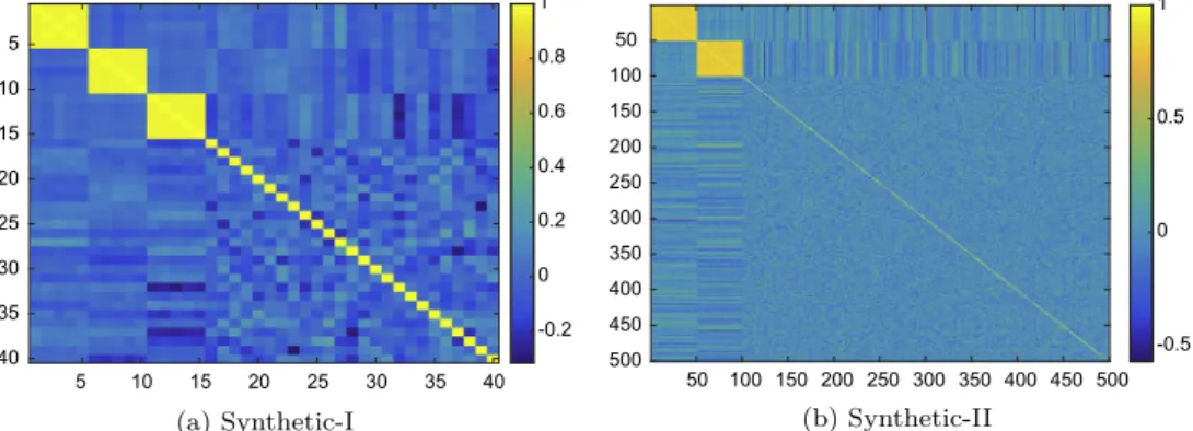
i are independent identically distributed N ð0;0:01Þ, i¼1;. . .;15. In this scenario, there are three equally important groups with five members within each group. The features within each group are strongly correlated. We expect these fea-tures to cause instability in feature selection process. This data-set has been used before in[16,47]. The empirical correlation matrix of this dataset is shown inFig. 5(a).

2. Synthetic-II: We simulate 100 datasets, each having 30=30=50 instances. In this simulation, we illustrate a situation ofp>n, withp¼500. The instances (rows ofD) are iid from aN ð0;RÞ

distribution, whereR is appblock diagonal matrix, which is defined as follows:

R

ij¼ 1 if i¼j; 0:8 if i50; j50; i–j; 0:8 if 516i100; 516j100; i–j; 0 otherwise 8 > > > < > > > : ð13Þ

and

i N ð0;2:52Þ,i¼1;. . .n. The true parameters are: w¼ 1_{|fflfflfflffl{zfflfflfflffl}};. . .;1 50 ;1_{|fflfflfflfflfflfflfflffl{zfflfflfflfflfflfflfflffl}};. . .;1 50 ;0_{|fflfflfflffl{zfflfflfflffl}};. . .;0 400 0 @ 1 A_:

In this scenario, there are two groups of 50 correlated features, which are associated with response. The remaining 400 features are uncorrelated and are not associated with response.Fig. 5(b) shows the empirical correlation matrix of this dataset.

3. Synthetic-III (simulation of microarray dataset): Analysis of microarray datasets is extremely useful for biomarker discovery and answering diagnosis and prognosis questions. In this sec-tion, we use a simulated dataset developed in[59]to compare the stability and prediction performance of pg-EN with other baseline algorithms. The effect of heterogeneity and variability of synthetic microarray data consisting of two balanced groups of 50 subjects is simulated in this dataset. To this end, each sub-ject is simulated using a regulatory network ofp= 10,000 genes using the simulator described in[60]. The topology of the net-work is specified by a connectivity matrixW, wherewijwould be non zero if gene-productjdirectly affects the expression of

gene i. Following this, a population of N¼1000 instances is simulated as follows. Subjects are modeled as regulatory net-works ofp= 10,000 nodes and the first generation of population consisted ofNindividuals with identical connectivity matrixW and withpdimensional vectors of expression values obtained. The subsequent generations were produced by iteration of three steps: random pairing, mutation of a randomly chosen subsequent of subjects and selection of the surviving subjects. These steps were applied only to a sub-network sizep¼900, indicated as W900in the following. These three steps are dis-cussed in more details in[59]. When the base population was simulated, we define two groups of 500 subjects. The patholog-ical condition is simulated by knocking out or knocking down six target hubs, which are defined as the genes with the highest out-degree and expression value at steady state higher than 0:88. Diseased subjects had 4, 5, or 6 genes belonging toW900 that were knocked out or down. In our studies, we partitioned the two groups of 500 healthy and 500 diseased subjects into 10 balanced non-overlapping datasets of size 50 subjects.

5.1.2. Real-world datasets

In order to show the effectiveness of our method for feature sta-bility on real-world problems we use three real datasets. Descrip-tion of each dataset is provided below:

Breast cancer dataset:This dataset was collected by Van De Vij-ver et al.[61]and consists of gene expression data for 8141 genes in 295 breast cancer tumors (87 metastatic and 217 non-metastatic).1

Cancer (EMR) dataset: This dataset is obtained from a large regional hospital in Australia.2 _{There are eleven different cancer}

types in this data recorded from patients visiting the hospital during 2010–2012. Patient data is acquired from Electronic Medical Records (EMR). The dataset consists of 4293 patients with 3867 variables including International Classification of Disease 10 (ICD-10), proce-dure and diagnosis related Group (DRG) codes of each patient as well as demographic data (age, gender and postcode). In this data set, the number of patients who survived within 1 year after diagnosis of cancer is 3383 and the number of those who died within 1 year is 910. Using this dataset, our goal is to predict 1 year mortality of patients while ensuring the stable feature sets. We note that feature stability is crucial for clinical decision making towards cancer prog-nosis. This dataset has been previously used in[13].

AMI (EMR) dataset:This dataset is also obtained from the same hospital in Australia. It involves patients admitted with AMI condi-tions and discharged later between 2007 and 2011. The task is to predict if a patient will be re-admitted to the hospital within Number of iterations 0 20 40 60 80 100 J ( ,G) 900 950 1000 1050 1100 1150 1200 1250 Cancer data Number of iterations 0 20 40 60 80 100 J ( ,G) 350 400 450 500 550 600 650 AMI data

Fig. 4.Empirical convergence of pg-EN for Cancer (EMR) and AMI (EMR) datasets.

1

Available at:http://cbio.ensmp.fr/ljacob.

2

(8)

30 days after discharge. The dataset consists of 2941 patients with 2504 variables include International Classification of Disease 10 (ICD-10), procedure and diagnosis-related Group (DRG) codes of each admission; details of procedures; and departments involved in the patient’s care. Other variables include demographic data and details of access to primary care facilities. In this data set the number of patients who are readmitted to the hospital within 30 days after discharge is 242 and those who are not readmitted are 2699. This dataset has been previously used in[13,62].

As these datasets are imbalanced, we balance them by using multiple replicates of each positive sample while keeping all repli-cates in the same fold during cross validation.

5.2. Baselines

To compare the performance of pg-EN with other state-of-the-art algorithms we have used the following algorithms as baseline. 5.2.1. Lasso

Lasso is a regularization method that is used to learn a regular-ized regression/classification model that is sparse in the feature space[7]. In a linear regression problem, Lasso uses al1-norm reg-ularization term that penalizes the sum of absolute value of weights. Its optimization function is as follows

arg min b 1 2kyXbk 2 2þkkbk1; ð14Þ

wherekis the non-negative tuning parameter. The solution of the above optimization does not have a closed form and is usually found iteratively by minimizing the cost function using pathwise coordinate optimization[54].

5.2.2. Elastic net

One of the limitations of Lasso in feature selection is that in presence of group of highly correlated features, it tends to select one feature among the group randomly and ignores the others. This renders Lasso to be unstable in feature selection. Elastic net tends to solve this problem by incorporating a quadratic part in the Lasso’s penalty term. The Elastic net cost function for a linear regression problem is as follows

arg min b 1 2kyXbk 2 2þkð1

a

Þk kb 1þk

a

2kbk 2 2; ð15Þ

where

a

2 ½0;1andkare tuning parameters. As a result, Elastic net includes Lasso and Ridge regression.

5.2.3. K-means+Lasso

In this baseline, we first useK-means to cluster the features and assign them to different groups based on their correlation. When

we prepare matrixG2RpK_{from the output of}_K_{-means. Each} col-umn ofGrepresents a group such that if featurepis part of groupk, then we haveGpk¼1 and 0 otherwise. We use this matrix to merge features which are in the same group. In particular, we obtain new feature matrixXfrom the original feature matrixDasX¼DG. Then usingX, we apply Lasso on it to obtain coefficientsb. In order to evaluate the stability of this method, we examine stability mea-sures (SRCC, JSM, and Kuncheva Index) on the coefficients of each individual feature obtained fromw¼Gb.

5.2.4. K-means+GroupLasso

Here, similar to the previous method, we cluster features using K-means and obtain the matrixG. To merge features which are in the same group, we obtain matrixX¼DG. Following this, we apply GroupLasso on the matrixXto obtain coefficientsbfor each group of features. To evaluate the stability ofK-means+GroupLasso, we examine stability measures on the coefficients obtained from w¼Gb. This method andK-means+Lasso are two examples that study the effect of unsupervised clustering to obtain groups of cor-related features.

5.2.5. Oscar

Octagonal shrinkage and clustering algorithm for regression (Oscar) is a penalized technique that study supervised clustering in linear regression. It simultaneously identifies a predictive group by assigning the same weights to each elements in the group up to a change in sign and eliminate redundant features. The cost func-tion of Oscar is as follows

1 2kyXbk 2 2þk1kbk1þk2 X 16j6k6p maxfbj;bkg; ð16Þ

wherek1andk2are non-negative tuning parameters. Thel1norm regularization term penalizes the sum of absolute value of weights and encourages sparsity.l1norm regularization term (max

opera-tor) encourages equality of the weights. 5.3. Evaluation measures

The proposed method and the baselines are evaluated in terms of their stability in feature selection and predictive performance. The evaluation measures are described below:

5.3.1. Stability measures

To compare the stability performance of pg-EN with other base-lines, we use three stability measures, Spearman’s rank correlation (SRCC), Jaccard similarity measure (JSM) and Kuncheva Index[50]. These stability measures are described in detail in Section3. 5 10 15 20 25 30 35 40 5 10 15 20 25 30 35 40 -0.2 0 0.2 0.4 0.6 0.8 1 50 100 150 200 250 300 350 400 450 500 50 100 150 200 250 300 350 400 450 500 -0.5 0 0.5 1

(9)

5.3.2. Predictive performance measures

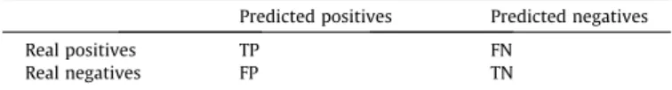
To compare the predictive performance of pg-EN with other baselines for regression problems (in Synthetic-I and Synthetic-II datasets) we use Mean Squared Error (MSE). For classification problems (Synthetic-III and real-world datasets), we use five eval-uation methods including Precision or Positive Predictive Value (PPV), Sensitivity, Specificity, F1 score and AUC. These evaluation methods are based on a confusion matrix, which is shown is Table 1.

Precision or PPV:Precision or Positive Predictive Value (PPV) is defined as the fraction of retrieved instances that are relevant i.e. PPV¼ TP

TPþFP: ð17Þ

Sensitivity or Recall:Sensitivity or recall measures the propor-tion of positives that are correctly identified i.e.

Sensitivity¼ TP

TPþFN: ð18Þ

Specificity:Specificity measures the proportion of negatives that are correctly identified i.e.

Specificity¼ TN

FPþTN: ð19Þ

F1 score:In some applications such as bioinformatics, datasets are imbalanced and number of examples belonging to one class is often lower than the overall number of examples. In this situa-tion, we are interested to mostly focus on one class (often positive class) and so we use the F1 score for this aim:

F1 score¼2 precision recall

precisionþrecall ; ð20Þ

Therefore, a high value of F1 score is better and ensures us that both precision and recall are reasonably high.

Area under the receiver operating characteristic curve (AUC):AUC is also commonly used to evaluate the performance of classifiers in imbalanced datasets and provides an approach for evaluating clas-sifiers based on an average which graphically interprets the perfor-mance of the classification algorithm by plotting the true positive rate against the false positive rate.

5.3.3. Statistical test

To determine whether there are significant differences between the results obtained using different algorithms on each dataset we perform statistical test. To this end, we use pairwise Wilcoxon signed-rank test (a non-parametric alternative to the paired t-test) with the significance level of 0:05 for every pair of models. We assume the null hypothesis statement as ‘‘both algorithms in the pair perform equally” and the alternative hypothesis statement as the opposite. So, if thep-value obtained from pairwise Wilcoxon signed-rank test is less than the significance level (¼0:05 in our study), then the null hypothesis is rejected. So, based on the pop-ulation mean of the model, we can conclude which model outper-forms the other.

5.4. Experimental settings

As mentioned in Section5.1.1for Synthetic-I and Synthetic-II, we simulate 100 datasets for each scenario, where each dataset consists of training set, validation set and test set. We fit the model on the training set and select parameters (tuning parameters in all the models and number of groups in pg-EN, KM+Lasso and KM +GroupLasso) using validation set. Then we evaluate its perfor-mance on the test set. The results for stability and prediction per-formance of each method are reported as an average over these 100 simulations.

For Synthetic-III, we partition two groups of 500 healthy and 500 diseased subjects into 10 balanced non-overlapping datasets of size 50 subjects. We do this procedure 10 times, so finally we will have 100 datasets of 50 subjects. We use external cross-validation loops with separate training and test phases. The final results are reported as an average over 100 datasets.

Turning to real datasets, we randomly divide data into training set and test set. All the models are trained on the training set and their performances are evaluated using the test set. Parameters of the models are selected using 5-fold cross validation on the train-ing set. The random splitttrain-ing of real datasets is done 100 times and the results (stability and predictive performances) are reported as an average over these 100 splits.

5.5. Experimental results

In this section we compare stability and predictive performance of pg-EN with other baseline regression and feature selection algorithms.

5.5.1. Stability performance

Table 2andFig. 6compare the stability performance of pg-EN with other baselines in terms of SRCC, JSM and Kuncheva Index. To this end, we examine these stability measures on coefficients of pg-EN obtained from w¼Gb. The numbers in brackets in Table 2 show the p-values obtained by applying Wilcoxon signed-rank test to the best and the second best stability results for each dataset.

For Synthetic-I the most stable method is pg-EN with SRCC = 0_:512 and JSM = 0_:627. In terms of SRCC the second best stability belongs to KM+Lasso (0:487) and in terms of JSM it belongs to Elastic net (0:620). The small p-values obtained from Wilcoxon signed-rank test also confirm that the there is significant difference between the stability obtained using pg-EN and the sec-ond best method. For Synthetic-II, In terms of SRCC again the most stable method is pg-EN (SRCC = 0:503), which is followed by Oscar (SRCC = 0:457). However, in terms of JSM, the stability perfor-mance of pg-EN is equivalent to Elastic net. In this case, the Wil-coxon test could not reject the null hypothesis. Turning to Synthetic-III (Microarray dataset) again pg-EN is the most stable method with SRCC = 0:487 and JSM = 0:587. In terms of SRCC, pg-EN is followed by Elastic net with SRCC = 0:402 and in terms of JSM it is followed by Oscar with JSM = 0:575.

In case ofBreast cancer dataset, the best stability performance in terms of SRCC belongs to Oscar (0:512), which is followed by pg-EN (0:502). However, in terms of JSM again pg-EN shows the best sta-bility (0:617), followed by Elastic net (0:583) and Oscar (0:580). In Cancer (EMR) dataset, pg-EN shows the best stability performance with SRCC = 0:543 and JSM = 0:622. In terms of SRCC, pg-EN is fol-lowed by Elastic net (0:443) and KM+GroupLasso (0:442), respec-tively. Turning to JSM, Oscar (0:530) and Elastic net (0:527) are in the next stages after pg-EN. ForAMI (EMR) dataset, once again pg-EN is the winner in terms of both SRCC (0:524) and JSM (0:614), followed by Oscar with SRCC = 0:467 and JSM = 0:552 and Elastic net with SRCC = 0:436 and JSM = 0:540. As seen from the table, for all datasets Lasso has the least stability performance in terms of both SRCC and JSM.

Table 1 Confusion matrix.

Predicted positives Predicted negatives

Real positives TP FN

(10)

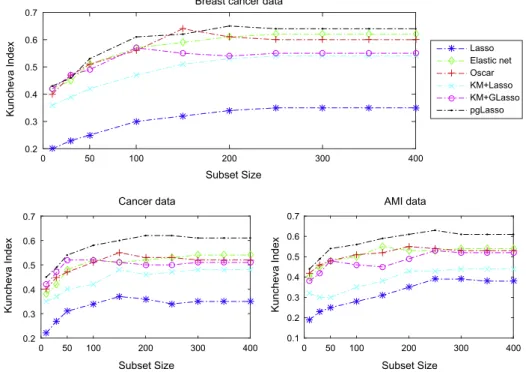
Fig. 6, compares the stability of pg-EN with other baselines in terms of Kuncheva Index on real-world datasets. As seen from this figure, the stability performance of pg-EN consistently outperforms other methods. Also, Lasso is the least stable method among others in all datasets. These results empirically demonstrate that pg-EN can greatly stabilize Lasso.

5.5.2. Predictive performance

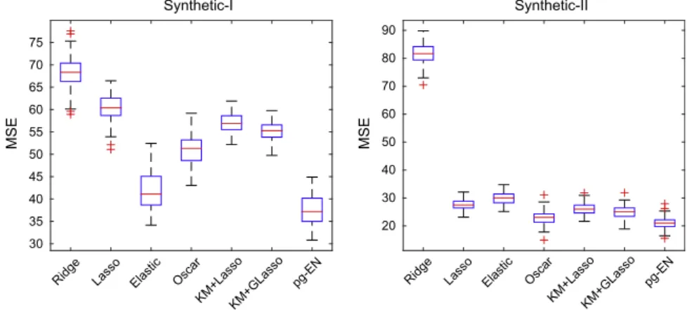
Fig. 7compares the predictive performance of pg-EN with other baselines on Synthetic-I and Synthetic-II datasets in terms of Mean Squared Error (MSE). We have also reported the statistical signifi-cance of each method inTable 3estimated using the pairwise Wil-coxon signed-rank test with significance level of 0:05. As seen from the box plots and thep-values inTable 3(a) and (b), pg-EN results in better predictive performance compared to other methods.

Table 4shows the predictive performance of pg-EN compared to other methods in terms of standard classification performances,

namely sensitivity, specificity, Positive Predictive Value (PPV), AUC scores and F1 score for the simulation of microarray dataset (Synthetic-III). Thep-values obtained from applying the Wilcoxon signed-rank test to the best and the second best classification mea-sures are also shown in brackets in the same table. As seen from Table 4pg-EN could obtain the best predictive performance among other methods. Thep-values also confirm that there is significant difference between the predictive performance of pg-EN and other baselines. We have also reported the statistical significance of comparisons between different algorithm pairs inTables 11 and 12inAppendix C.

Tables 5–7show the capability and effectiveness of the pg-EN compared to the baseline algorithms in terms of standard classifi-cation performances, sensitivity, specificity, Positive Predictive Value (PPV), AUC scores and F1 score for Breast Cancer, Cancer (EMR) and AMI (EMR) datasets, respectively. The numbers in brackets in each table show thep-values obtained by applying

Table 2

Average stability performance of pg-EN compared to other baselines in terms of SRCC and JSM, for synthetic and real datasets. The numbers in brackets show thep-values obtained by applying Wilcoxon signed-rank test to the best and the second best stability results for each dataset.

Synthetic data Real data

Syn-I Syn-II Syn-III Breast cancer Cancer AMI

Lasso SRCC 0.265 0.214 0.206 0.178 0.216 0.287 JSM 0.386 0.302 0.355 0.396 0.374 0.387 Elastic net SRCC 0.453 0.422 0.402 0.486 0.443 0.436 JSM 0.620 0.602 0.572 0.583 0.527 0.540 Oscar SRCC 0.482 0.457 0.398 0.512 0.426 0.467 JSM 0.602 0.577 0.575 0.580 0.530 0.552 KM Lasso SRCC 0.487 0.392 0.416 0.427 0.372 0.386 JSM 0.527 0.507 0.497 0.518 0.493 0.487 KM GLasso SRCC 0.326 0.387 0.376 0.462 0.442 0.437 JSM 0.552 0.519 0.543 0.531 0.516 0.510 pg-EN SRCC 0.512 0.503 0.487 0.502 0.543 0.524

(1.8e31) (1.0e26) (2.3e32) (0.017) (2.5e34) (1.5e28)

JSM 0.627 0.602 0.587 0.617 0.622 0.614

(3.6e24) (0.565) (1.7e09) (8.2e21) (7.8e33) (1.0e27)

The best performances are shown in bold.

Subset Size 0 50 100 200 300 400 Kuncheva Index 0.2 0.3 0.4 0.5 0.6 0.7 Cancer data Subset Size 0 50 100 200 300 400 Kuncheva Index 0.1 0.2 0.3 0.4 0.5 0.6 0.7 AMI data Subset Size 0 50 100 200 300 400 Kuncheva Index 0.2 0.3 0.4 0.5 0.6 0.7

Breast cancer data

Lasso Elastic net Oscar KM+Lasso KM+GLasso pgLasso

(11)

Ridge Lasso Elastic Oscar KM+Lasso_KM+GLasso pg-EN MSE 30 35 40 45 50 55 60 65 70 75 Synthetic-I

Ridge Lasso Elastic Oscar KM+Lasso KM+GLasso pg-EN MSE 20 30 40 50 60 70 80 90 Synthetic-II

Fig. 7.Comparing the prediction performance of pg-EN and other baselines on Synthetic datasets.

Table 3

Thep-value obtained from pairwise Wilcoxon signed-rank test of MSE applied to the Synthetic datasets (a) Synthetic_I and (b) Synthetic_II.

p-value Lasso Elastic net Oscar KM+Lasso KM+GLasso pg-EN

(a)

Ridge 5.17e17 4.73e18 5.87e18 5.95e15 3.64e17 3.89e18

Lasso 3.76e18 5.59e18 3.22e05 0.4432 4.26e18

Elastic net 5.11e18 3.75e18 4.27e18 4.86e10

Oscar 5.18e17 6.02e17 3.89e18

KM+Lasso 3.05e04 4.23e18

KM+GLasso 3.93e18

(b)

Ridge 4.23e18 5.01e18 3.98e18 4.10e18 4.05e18 3.88e18

Lasso 3.62e11 5.32e17 2.74e17 1.34e12 4.67e18

Elastic net 8.26e18 1.63e15 1.41e17 3.89e18

Oscar 3.02e12 1.49e12 1.43e07

KM+Lasso 0.0010 1.41e17

KM+GLasso 3.09e16

Table 4

Average classification performances of pg-EN compared to other methods for Synthetic-III dataset. The numbers in brackets show the p-values obtained by applying Wilcoxon signed-rank test to the best and the second best classification results for each dataset.

PPV Sensitivity F1 score Specificity AUC

Ridge 0.785 0.799 0.792 0.810 0.759 Lasso 0.821 0.815 0.818 0.833 0.787 Elastic net 0.823 0.819 0.821 0.856 0.792 Oscar 0.834 0.83 0.832 0.865 0.81 KM+Lasso 0.815 0.819 0.817 0.838 0.792 KM+GLasso 0.825 0.825 0.825 0.858 0.790 pg-EN 0.843 0.840 0.842 0.872 0.821 (0.003) (0.003) (0.004) (1.8e04) (0.003) The best performances are shown in bold.

Table 5

Average classification performance of pg-EN compared to other methods for Breast cancer dataset. The numbers in brackets show thep-values obtained by applying Wilcoxon signed-rank test to the best and the second best classification results for each dataset.

Table 6

Average classification performance of pg-EN compared to other methods for Cancer (EMR) dataset. The numbers in brackets show thep-values obtained by applying Wilcoxon signed-rank test to the best and the second best classification results for each dataset.

Table 7

Average classification performance of pg-EN compared to other methods for AMI (EMR) dataset. The numbers in brackets show thep-values obtained by applying Wilcoxon signed-rank test to the best and the second best classification results for each dataset.

Ridge 0.296 0.389 0.336 0.75 0.602 Lasso 0.309 0.400 0.348 0.756 0.608 Elastic net 0.31 0.403 0.35 0.758 0.61 Oscar 0.315 0.406 0.355 0.763 0.613 KM+Lasso 0.307 0.399 0.347 0.743 0.607 KM+GLasso 0.311 0.405 0.351 0.76 0.609 pg-EN 0.315 0.419 0.359 0.773 0.626 (0.7) (0.001) (3.3e04) (0.033) (1.0e05) The best performances are shown in bold.

(12)

Wilcoxon signed-rank test to the best and the second best classifi-cation results for each dataset.

For the Breast cancer dataset,Table 5shows that the best clas-sification performance in terms of all the clasclas-sification measures belongs to pg-EN with PPV = 0:325, Sensitivity = 0:309, F1 score = 0:429, Specificity = 0:898 and AUC = 0:855. This is Also con-firmed by thep-values obtained from pairwise Wilcoxon signed-rank test shown in brackets. The statistical significance of compar-isons between different algorithm pairs are presented inTables 13 and 14inAppendix C.

Table 6, compares the classification performance of pg-EN with other baselines on Cancer (EMR) dataset. As seen, again pg-EN could achieve the best predictive performance among other meth-ods with PPV = 0:323, Sensitivity = 0:392, Specificity = 0:831 and AUC = 0:728. This is also confirmed by thep-values obtained from pairwise Wilcoxon signed-rank test. However, in terms of F1 score, statistical test could not reject the null hypothesis and the perfor-mance of pg-EN and Oscar are comparable based on this classifica-tion measure. We have also reported the statistical significance of

comparisons between different algorithm pairs inTables 15 and 16 inAppendix C.

Table 7, shows the classification performance of pg-EN compare to other baseline algorithms on AMI (EMR) dataset. As seen, again pg-EN is the winner among other methods with Sensitivity = 0:419, F1 score = 0:359, Specificity = 0:773 and AUC = 0:626. This superi-ority is also confirmed by the statistical test. However, in terms of PPV, the performance of pg-EN is comparable with that of Oscar. The statistical significance of comparisons between different algo-rithm pairs are shown inTables 17 and 18inAppendix C. 5.5.3. Execution time

In Section4.1.2, we discussed about the computational com-plexity of pg-EN. Now, we empi+rically compare its execution time with some of the baseline methods on real-world datasets. All the experiments were executed on a Windows machine with 2.5 GHz Intel C600 chipset and 16 GB RAM. The obtained results inTable 8, show that the execution time of pg-EN is bigger than Lasso and Elastic net but it is less than Oscar. Also,Fig. 8, shows the execution time of pg-EN (using Cancer (EMR) dataset) comparing it with those of Lasso and Oscar for increasing number of samples. As shown, again the execution time of pg-EN is bigger than Lasso and lower than Oscar. Also, it is roughly linear in the number of samples, which suggests that pg-EN scales well on large datasets. 5.5.4. Effect of grouping

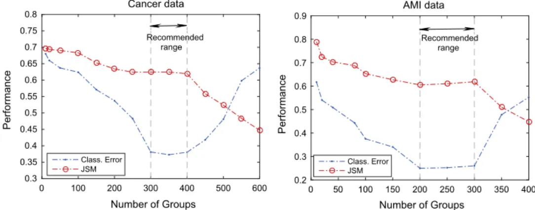
Fig. 9shows the prediction performance (in terms of classifica-tion error) and the stability performance (in terms of JSM) of pg-EN with respect to variation in number of groups for Cancer (EMR) and AMI (EMR) data. As seen from the left figure for Cancer data, when we decrease the number of feature groups in the model from around 600 to 300, both the stability and prediction performance improve. However, decreasing the number of groups further, even enforces lowly correlated features to be grouped together, which is almost acceptable for obtaining better stability, but degrades the prediction performance. Similar behavior is observed for AMI data-set. This suggest that one should not over-enforce the feature grouping. Therefore, the best number of groups in the model can be selected when there is a logical trade-off between prediction and stability performances. The recommended range for selecting the best number of groups in each dataset is shown by vertical lines inFig. 9.

5.5.5. Feasibility of grouping

Since for AMI data we have the detail information about feature names, we have shown some examples of feature groups estimated using pg-EN for this dataset inFig. 10. As seen from these figures,

Table 8

Execution time (in seconds) of pg-EN compared to some other methods for real datasets.

Dataset Lasso Elastic net Oscar pg-EN

Breast cancer 76.6 71.4 170.4 90.9

Cancer (EMR) 52.9 54.3 121.9 87.1

AMI (EMR) 48.3 50.2 107.8 69.3

The number of samples

1000 1500 2000 2500 3000 3500 4000 4500

Execution time (sec)

0 20 40 60 80 100 120 140 Lasso pg-EN Oscar

Fig. 8.Execution time (in seconds) of pg-EN compared to Lasso and Oscar on for different number of samples on Cancer (EMR) dataset.

Number of Groups 0 100 200 300 400 500 600 Performance 0.3 0.35 0.4 0.45 0.5 0.55 0.6 0.65 0.7 0.75 0.8 Cancer data Class. Error JSM Number of Groups 0 50 100 150 200 250 300 350 400 Performance 0.2 0.3 0.4 0.5 0.6 0.7 0.8 0.9 AMI data Class. Error JSM Recommended range Recommended range

Fig. 9.Prediction and stability performance of the model with respect to variation in number of groups, shown for Cancer and AMI datasets. The recommended range for number of groups is marked by vertical lines.

(13)

features in each group are related to a special type of disorder. The features shown inFig. 10(a), are all related tobone diseases, features that are listed inFig. 10(b), are related tocardio-pulmonary diseases. Fig. 10(c) shows the features of psycho-emotional disorders and

Fig. 10(d) lists the features, related tobrain diseases. We note that in these figures the features which are associated with suffixes 3M, 6M or 1Y, show that those features occurred in previous 3 months, or 6 months or 1 year of prediction.

We have also assessed the grouping ability of pg-EN on Soil data, which studies relation between soil characteristics and rich-cove forest diversity in the Appalachian mountains of North Carolina. Although this dataset is non-medical, its small number but highly correlated features allows for an in-depth illustration of the behavior of our proposed model. The explanation and obtained results related to this dataset is presented inAppendix A. 5.5.6. Risk factors obtained using pg-EN

As mentioned before, identifying robust variables can assist domain experts in their decision makings towards accurate medi-cal prognosis. InTables 9 and 10we have reported some of the top variables obtained using pg-EN for Cancer and AMI datasets. The importance of these variables is based on the predictive weights assigned to them by the pg-EN. To select the top risk factors, we use the feature sets obtained by 100 splitting of the data and com-pute the mean weights of the selected variables over these 100 splits and some of the variables with highest absolute weights are reported in the Table. Also, we empirically estimate the proba-bility of presencefor each feature. In these tables, column 1 shows the variable’s name, Column 2 shows its ICD-10 code, Column 3 shows its average weight and Column 4 shows it probability of presence in data splits.

6. Conclusion

We have proposed a new model to stabilize Lasso in selecting informative features, which is crucial in applications such as Healthcare and bioinformatics where the features carry intuitive meanings and interpreting informative features is important in decision makings. The model learns a grouping of correlated vari-ables using supervised data and performs feature selection,

simul-Fig. 10.Example of feature groups obtained using pg-EN for AMI data. Features in a group are consistent and related to (a) bone, (b) cardio-pulmonary, (c) psycho-emotional and (d) brain diseases. Features which are associated with suffixes 3M, 6M or 1Y, show that those features occurred in previous 3 months, or 6 months or 1 year of prediction.

Table 9

Top selected variables for cancer obtained by pg-EN are consistent with the risk factors reported by expert domains and other research papers.

Risk factor ICD-10

code Weights Probability of presence Benign neoplasm of breast D24[63] 0.0715 ± 0.0010 0.92 Type II diabetes mellitus E11 [64,65] 0.0627 ± 0.0021 0.84 Anorexia R63.0 [66] 0.0601 ± 0.0014 0.82 Nausea and vomiting R11

[67,65] 0.0502 ± 0.0011 1 Fatigue R53[65] 0.0426 ± 0.0024 1 Diarrhea R19.7 [67] 0.0402 ± 0.0016 0.86 Table 10

Top selected variables for readmission after AMI obtained by pg-EN are consistent with the variables reported by expert domains and other research papers.

Risk factor ICD-10 code Weights Probability of presence Angina pectoris I20[68,69] 0.0743 ± 0.0010 0.98 Kidney disease N17, N18 [70,69,71] 0.0616 ± 0.0006 0.78 Diabetes and DM complications E10, E11 [70,69] 0.0545 ± 0.0002 0.75 COPD J44[70,69] 0.0525 ± 0.0012 0.79 Hypertension I10[72,70,73] 0.0516 ± 0.0023 0.88 Cardio-respiratory failure E83.4[74] 0.0432 ± 0.0017 0.85

(14)

taneously. The model is formulated as a constrained optimization problem that can jointly learn feature groups and their relevance. Also, an iterative optimization algorithm is proposed that can effi-ciently solve the problem with theoretical guarantee on conver-gence. We compare the stability and prediction performance of the proposed method with several state-of-the-art regression and feature selection methods namely, Ridge regression, Lasso, Elastic net, Oscar,K-means+Lasso and K-means+GroupLasso using three synthetic and three real-world datasets (Breast cancer data, Cancer (EMR) data and AMI (EMR) data). We show that as the proposed model learns groups of correlated features and performs feature selection based on these groups, its feature selection stability is notably better than Lasso and comparable to other methods. In terms of prediction performance, we also show that the proposed model leads to better results than baseline algorithms. This is due to estimator’s variance reduction that itself is the result of grouping correlated features. Our results can be applied to identify stable risk factors for many problems in healthcare domain and bioinformatics and therefore can assist clinicians and domain experts in their decision makings towards more accurate medical prognosis.

Conflict of interest

The authors declared that there is no conflict of interest. Appendix A. Grouping results on Soil data set

In order to show that our model yields feasible groups, we assess our model on a small dataset called Soil data[16]. This data-set studies relation between soil characteristics and rich-cove for-est diversity in the Appalachian mountains of North Carolina. Twenty 500-m2_{plots were surveyed. The outcome shows the} num-ber of different plant species found in the plot. 15 soil characteris-tics are used as variables to predict forest diversity and are shown inFig. 11. As it can be seen from this figure, there are groups of highly correlated variables. The first seven variables that are all related to cations are highly correlated. Sodium and phosphorus are also highly correlated as well as soil pH and exchangeable acid-ity, which are measures of acidity. In addition, as the sum of cations can be derived through sum of all cations namely, calcium, magnesium, potassium, and sodium, the design matrix is not full rank. Fig. 12 shows the obtained grouping matrix (GÞ using pg-EN for Soil data. As it is shown in this figure, the obtained grouping matrix of the features is sparse and also there are no overlaps between groups. It also shows the ability of pg-EN in selecting and grouping correlated features. As mentioned earlier, in order to increase the stability and predictive performance of the model, unlike Lasso that treats each variable separately and randomly selects a representative, pg-EN tends to use the group of correlated features and treat them as a derived variable. As the figure shows, pg-EN could group the four selected cation variables together i.e. percent base saturation (BaseSat), sum of cations (SumCation), cal-cium (Ca) and magnesium (Mg). It could also group acidity-related variables i.e. pH and exchangeable acidity (ExchAc). The algorithm assigns a unique weight (b) to each group. Because highly corre-lated variables have the same underlying factor, supervised group-ing of these variables can result in better estimation of the underlying factor of correlated variables and present more infor-mative predictive model.

Appendix B. Proofs B.1. Proof ofProposition 1

Proof.We define the Lagrangian function

LðGÞ ¼trð2bTGTDTyþbTGTDTDGbdGTG

_l

GTÞ; ð:1Þ where the Lagrangian multipliers

_l

_ij introduce nonnegative con-straints,GP0. From the zero gradient condition

@L

@G¼ 2D T_y

bTþ2DT_DG

bbT2dG

_l

¼0: From the complementary slackness condition,

ð2DTybTþ2DTDGbbT2dGÞikGik¼

l

ikGik¼0: ð:2Þ

This is the fixed point equation, and we show that the limiting solu-tion of the update rule of(10)satisfies this equation. At conver-gence,G1¼Gðtþ1Þ¼GðtÞ¼G, so Gik¼Gik ffiffiffiffiffiffiffiffiffiffiffiffiffiffiffiffiffiffiffiffiffiffiffiffiffiffiffiffiffiffiffiffiffiffiffiffiffiffiffiffiffiffiffiffiffiffiffiffiffiffiffiffiffiffiffiffiffiffiffiffiffiffiffiffiffiffiffiffiffiffiffiffiffiffiffi BGAþ ikþ B þ_GA ikþC þ ikþdGik BþGAþ ikþ B _GA ð ÞikþC ik s ; ð:3Þ where A¼bbT; B¼DT_D_; _C_¼_DT_y bT. AsB¼BþB; A¼AþA, hence we haveBGA¼ BþBG AþA. Thus,(.3)reduces to

−1 −0.8 −0.6 −0.4 −0.2 0 0.2 0.4 0.6 0.8 1 BaseSat SumCation CECb

uff

er

Ca Mg K Na P Cu Zn Mn HumicMatter Density pH ExchAc BaseSat SumCation CECbuffer Ca Mg K Na P Cu Zn Mn HumicMatter Density pH ExchAc

Fig. 11.Computed feature correlation matrix for Soil data.

Obtained grouping matrix for soil data

Group number 1 2 3 4 5 BaseSat SumCation CECbuffer Ca Mg K Na P Cu Zn Mn HumicMatter Density pH ExchAc -1 -0.8 -0.6 -0.4 -0.2 0 0.2 0.4 0.6 0.8 1

Fig. 12.Group matrix obtained for Soil dataset. (The groups numbers are permuted to assist comparison withFig. 11.)

(15)

ð2DTybTþ2DTDGbbT2dGÞikG

2

ik¼0: ð:4Þ

Eqs.(.4) and (.2)are identical. Both the equations require that at least one of the two factors is equal to zero. The first factor in both equations is identical. For the second factorGik andG2ik, ifGik¼0, thenG2

ik¼0, and vice versa. Thus, if(.2)holds then(.4)also holds and vice versa. In the following propositions we prove that the iter-ative update algorithm converges. h

B.2. Proof ofProposition 2

Proof.We can writeJðHÞas

JðHÞ ¼trð2HTCþþ2HTCþAþHTBþHAþHTBH

AHT_Bþ_H_þ_A_HT_B_H_d_HT_H_Þ_; _ð_:_5Þ

whereA¼bbT; B¼DT_D

; C¼DT_y

bT, andH¼G. We use an auxil-iary function approach similar to that used in[55,56].ZðH;H0Þis an auxiliary function of JðHÞ if it satisfies ZðH;H0ÞPJðHÞ and ZðH;HÞ ¼JðHÞ, for anyH;H0. We define the update rule

Hðtþ1Þ_¼_{arg min} H ZðH;H

ðtÞ_Þ_; _ð_:_6Þ

whereJðHðtÞ_{Þ ¼}_Z_ð_HðtÞ_;_HðtÞ_Þ_P_Z_ð_Hðtþ1Þ_;_HðtÞ_Þ_P_J_ð_Hðtþ1Þ_Þ_{. Hence,}_J_ð_HðtÞ_Þ

is non-increasing. So we should find an appropriateZðH;H0Þand its global minimum. InProposition 3, we defineZðH;H0Þas an auxiliary function ofJthat its minimum is(12). According to(.6),Hðtþ1Þ

H andHðtÞ

H0; replacingH¼G, we obtain(9). h B.3. Proof ofProposition 3

Proof.We find upper bounds for positive terms and lower bounds for negative terms. For the second term inJðHÞ, we have an upper bound trðHTCÞ ¼X ik HikCik6C ik H2 ikþH 02 ik 2H0ik ; using inequalitya6ða2_þ_b2_Þ

=2a. The third and sixth terms inJðHÞ, are bounded by trðAþHT_Bþ_H_Þ₆X ik ðBþH0AþÞikH 2 ik H0ik ; trðAHT_B_H_Þ₆X ik ðBH0AÞikH 2 ik H0_ik ;

using Proposition 4. Lower bounds for the remaining terms are obtained using the inequalityzP1þlogðzÞ, which is true for any z>0. We obtain Hik H0ik P1þlogHik H0ik ; HikHil H0ikH 0 il P1þlogHikHil H0ikH 0 il ð:7Þ Using(.7), we can bound the first, fourth, fifth and last terms ofJðHÞ

as follows trðHT_Cþ_Þ_PX ik CþikH 0 ik 1þlog Hik H0ik ; trðAþHTBHÞPX i;j;k;l BijH0jkA þ klH0il 1þlog HjkHil H0jkH 0 il ! ; trðAHTBþHÞPX i;j;k;l BþijH 0 jkA klH 0 il 1þlog HjkHil H0jkH 0 il ! ; trðHT_H_Þ_PX i;k;l H0ikH0il 1þlog HikHil H0ikH 0 il :

We can obtainZðH;H0Þas in(11), by collecting all bounds. It is obvi-ous thatJðHÞ6ZðH;H0ÞandJðHÞ ¼ZðH;HÞ. To find the minimum of ZðH;H0Þ, we take @ZðH;H0Þ @Hik ¼ 2CþikH 0 ik Hik þ2C ikHik H0ik þ2 B þ_H0_Aþ ikHik H0ik 2 B _HAþ ikH 0 ik Hik 2 B þ_HA ikH 0 ik Hik þ2 B _H0_A ikHik H0ik d2H 0 ik Hik :

The Hessian ofZðH;H0Þis written by noting@_@2_HZðH;H0Þ

ik@Hjl ¼dijdklZikwhere Zik¼ 2 Cþikþ B _H0_Aþ ikþ B þ_H0_A ikþd H0ik H2 ik þ2C ikþ B þ_H0_Aþ ikþ B _H0_A ik H0ik :

This matrix is a diagonal matrix with positive entries. We infer that ZðH;H0Þis a convex function ofH. If we solve@ZðH;H0Þ

@Hik ¼0 forH, we

recover(12). h

Proposition 4. For any matrices P2Rnn

þ , R2Rkþk, S2Rnþk and

S02Rnk

þ , with symmetric P and R we have

trðST_PSR_Þ₆X n i¼1 Xk j¼1 ðPS0RÞijS 2 ij S0_ij : ð8Þ

Proof. IfSij¼S0ijuij, the difference between the left-hand side and the right hand side can be written as

D

¼X n i;t¼1 Xk j;q¼1 PijS0tqBqjS0ijðu 2 ijuijutqÞ:

AsPandRare symmetric, this is equal to

D

¼X n i;t¼1 Xk j;q¼1 PijS0tqBqjS0ij u2 ijþu 2 tq 2 uijutq ! ¼1 2 Xn i;t¼1 Xk j;q¼1 PijS0tqBqjS0ijðuijutqÞ 2 P0:

Appendix C. Statistical test results

As mentioned in the paper, in order to have a better comparison between the results obtained using our proposed method and other baselines, we have performed pairwise Wilcoxon signed-rank test with significance level of 0:05 for each prediction mea-sure. Thep-values obtained from this statistical test are shown in Tables 11–18for Synthetic-III (Microarray), Breast cancer, Cancer (EMR) and AMI (EMR) datasets.