Munich Personal RePEc Archive
A Residual-Based Cointegration test
with a Fourier Approximation
Yilanci, Veli
Sakarya University
31 July 2019
Online at
https://mpra.ub.uni-muenchen.de/95395/
A Residual-Based Cointegration test with a Fourier Approximation
Veli YILANCI*
*a
Corresponding Author; Department of Econometrics, Sakarya University, Sakarya, Turkey,
https://orcid.org/0000-0001-5738-690X,[email protected].
Abstract
This paper proposes a residual-based cointegration test in the presence of smooth structural
changes approximated by a Fourier function. The test offers a simple way to accommodate
unknown number and form of structural breaks and have good size and power properties in the
presence of breaks.
Keywords: cointegration test; Fourier function; structural breaks.
JEL Codes: C12, E4.
1. Introduction
The performance of traditional residual-based cointegration tests that examine the null
hypothesis of the nonexistence of a long-term relationship between economic variables is affected
by structural changes that occur due to economic crises, technological changes, political regime
shifts, and similar shocks. As noted by Gregory and Hansen (1996), if structural breaks exist, the
power of cointegration tests, such as Engle-Granger (1987), which ignore these changes, will be
reduced. Several cointegration tests have been introduced to take into account structural breaks
in the cointegration relationship. While Gregory and Hansen (1996) considered one unknown
shift, Hatemi-J (2008) extended this test to allow two structural breaks. Both of the tests capture
the regime shifts incorporating dummy variables and assume the number of breaks a priori.
The study by Becker et al. (2005, BEL hereafter), who used Gallant’s Flexible Fourier form to
model unknown structural breaks, brought new depth to the unit root testing literature because
previous studies generally used Perron’s (1989) modeling strategy of structural breaks with
dummy variables. BEL (2005) showed that a single frequency of Fourier approximation can mimic
various breaks and unattended nonlinearity. Several unit root tests, such as those by BEL (2005),
Enders and Lee (2012), and Rodriguez and Taylor (2012), who employed a variant of the Flexible
Fourier form, have been introduced to the literature. The main advantage of using trigonometric
terms is that the locations, numbers, and forms of the structural breaks do not need to be
predetermined. In this study, we extend the residual-based cointegration test of Engle-Granger
(1987) using Fourier approximation to test the existence of a cointegration relationship allowing
unknown forms of breaks. The remainder of the paper is organized as follows: Section 2 defines
the model and test statistic and contains the asymptotic distributions of the latter; Section 3
assesses the size and power of the suggested test statistic; and, finally, Section 4 presents the
2. Model with Fourier Approximation and Test Statistics
We consider the following cointegration regression in this paper:
1t
'
2t ty
d t
y
u
(1)where
t
1, 2,...,
T
. The dependent variabley
t is a scalar, andx
t
x
1t,...,
x
mt
'
is a
m
1
vector of independent variables.
d t
is a deterministic function of t that can be approximatedusing the following Fourier expansion with a single-frequency component1:
02 2 sin cos k k kt kt d t T T
where
0 shows the traditional deterministic term including a constant with or without a linearterm,
T
shows the number of observations, and k represents the Fourier frequency, the valuesof which are selected using the value that minimizes the sum of squared residuals (SSR). When
0
k k
, there is no nonlinear trend, and the traditional Engle-Granger cointegration testemerges.
We obtain the following equation when we implement this function in Model 1:
1 0 1 2 2
2 2
sin cos '
t t t
kt kt
y y u
T T
(2)
To test the null hypothesis of no-cointegration, we apply the Augmented Dickey-Fuller unit root
test to the residuals of Model 2. Hence, we estimate the following autoregression:
1 1
ˆt ˆt p iˆt i t i
u
u
u
1 It is also possible to use multiple frequencies in the Fourier expansion; to conserve space, the critical values
Where
t ~ . . . 0,i i d
2
, we let
FEG show the t-statistics for the null hypothesis ofno-cointegration that is defined as:
ˆˆ FEG se
where
ˆ
denotes the ordinary least squares estimator of
whilese
ˆ
is the standard error ofˆ
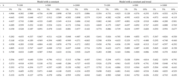
.Critical values for the Fourier cointegration test (FEG) are obtained via simulations considering a
different number of regressors (n = 1, 2, 3) and frequency values (k = 1, 2, 3, 4, 5). We report them
in Table 1, considering both constant, and constant and trend cases for the sample sizes are t =
100, 500, and 1000.
[Table 1 about here]
As can be seen in Table 1, the asymptotic distribution of the test statistic depends on the frequency
(k) and number of regressors (n). While ceteris paribus, an increase in k and/or n creates a
decrease in critical values.
3. Size and power properties
We analyzed the finite sample properties of the suggested test by considering the following data
generation process (DGP):
1 0 1 2 1 1, 1 2 1 2 1
2 2
sin cos ,
t t t t t
kt kt
y y y y
T T
2t 2t 1 2t
,
y
y
2 1 12 2 21 2 . t tE
where
t
1t, 2t
,1
2 2
1 yt
and2
2 2
2 yt
. We assume that
1
and
12
21
. SimilarDGPs have been used in several prior studies [see Banerjee and Smith (1986), Lee et al. (2015),
Banerjee et al. (2017) among others.]. We conducted simulations using 20,000 replications at the
5% significance level. We examined the performance of the test from different perspectives:
- we let the persistent measure
change in the range {0, 0.9};- we set
12 1, while letting the 2 2
vary along with
1,16 ; and,- we also evaluate two sets of
1, and
2 as
1
0, 3
and
2
0,5
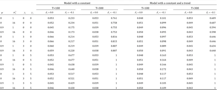
.We report the results in Table 2.
[Table 2 about here]
The results show that, as the sample size increases, the power of the test also increases2. Besides,
in the case of
1
2
0
, when the magnitude of the break increases, the power of the FEG testincreases, and becomes 1, in most cases. When the persistent measure
increases, the power ofthe test seems to decrease in the case of
1
2
0
. In this case, an increase in 22 causes anincrease in the power of the test, in most cases. Overall, the test seems to have small size distortions
and good power properties in the existence of breaks.
2 Conventional Engle-Granger (1987) cointegration test loses power, and suffers from size distortions in
4. Conclusion
In this paper, we proposed a residual-based test for cointegration with a Fourier approximation
using a single-frequency component, allowing multiple smooth breaks. Thanks to the FEG
cointegration test, we do not need to know the exact location, form, or number of breaks a priori.
The only value to be determined is the frequency value, which is found by minimizing SSR. The
suggested test can prevent potential loss of power in the cointegration tests that allow structural
breaks by adding dummy variables in the testing equations. Simulation results show that the FEG
test has small size distortions and good power properties, especially in the existence of breaks.
References
Banerjee, P., Arčabić, V., & Lee, H. (2017). Fourier ADL cointegration test to approximate smooth
breaks with new evidence from crude oil market. Economic Modelling, 67, 114-124.
Banerjee, A., Dolado, J. J., Hendry, D. F., & Smith, G. W. (1986). Exploring equilibrium relationships
in econometrics through static models: some Monte Carlo evidence. Oxford Bulletin of Economics
and statistics, 48(3), 253-277.
Becker, R., Enders, W., Lee, J., 2006. A stationarity test in the presence of an unknown number of
smooth breaks. Journal of Time Series Analysis 27, 381–409.
Engle, R., Granger, C., 1987. Co-integration and error correction: representation, estimation, and
testing. Econometrica. 55 (2), 251–276.
Gallant, R., 1981. On the basis in flexible functional form and an essentially unbiased form: the
flexible Fourier form. Journal of Econometrics 15, 211–353.
Gregory, A. W., & Hansen, B. E. (1996). Residual-based tests for cointegration in models with
Hatemi-j, A. (2008). Tests for cointegration with two unknown regime shifts with an application
to financial market integration. Empirical Economics, 35(3), 497-505.
Lee, H., Lee, J., & Im, K. (2015). More powerful cointegration tests with non-normal errors. Studies
in Nonlinear Dynamics & Econometrics, 19(4), 397-413.
Leybourne, S., Newbold, P., 2003. Spurious rejections by cointegration tests induced by structural
breaks. Appl. Econ. 35, 1117–1121
Perron, P., 1989. The great crash, the oil price shock, and the unit root hypothesis. Econometrica
57, 1361–1401
Rodrigues, Paulo MM, and AM Robert Taylor. "The Flexible Fourier Form and Local Generalised
Least Squares De‐trended Unit Root Tests." Oxford Bulletin of Economics and Statistics74.5 (2012):
Table 1: Critical Values of FEG Cointegration Test
Model with a constant Model with a constant and trend
n k T=100 t=500 t=1000 T=100 t=500 t=1000
1% 5% 10% 1% 5% 10% 1% 5% 10% 1% 5% 10% 1% 5% 10% 1% 5% 10%
1 1 -4.906 -4.302 -3.988 -4.756 -4.198 -3.898 -4.738 -4.175 -3.886 -5.354 -4.731 -4.423 -5.128 -4.576 -4.293 -5.074 -4.555 -4.274
2 -4.665 -3.995 -3.648 -4.517 -3.912 -3.589 -4.503 -3.898 -3.579 -5.243 -4.582 -4.250 -4.995 -4.433 -4.136 -4.973 -4.410 -4.119
3 -4.437 -3.743 -3.380 -4.333 -3.685 -3.349 -4.314 -3.686 -3.342 -5.002 -4.340 -3.997 -4.801 -4.230 -3.910 -4.804 -4.208 -3.901
4 -4.285 -3.599 -3.252 -4.183 -3.554 -3.231 -4.172 -3.546 -3.221 -4.849 -4.175 -3.827 -4.697 -4.092 -3.767 -4.693 -4.088 -3.769
5 -4.190 -3.520 -3.187 -4.091 -3.478 -3.165 -4.081 -3.477 -3.165 -4.774 -4.086 -3.739 -4.634 -3.997 -3.683 -4.593 -3.994 -3.677
2 1 -5.282 -4.655 -4.337 -5.067 -4.511 -4.220 -5.048 -4.487 -4.205 -5.641 -5.026 -4.705 -5.404 -4.855 -4.571 -5.367 -4.826 -4.550
2 -5.168 -4.526 -4.189 -4.969 -4.394 -4.085 -4.949 -4.371 -4.065 -5.598 -4.954 -4.633 -5.329 -4.772 -4.480 -5.295 -4.748 -4.460
3 -4.958 -4.283 -3.938 -4.804 -4.183 -3.870 -4.778 -4.172 -3.852 -5.450 -4.781 -4.436 -5.199 4.620 -4.313 -5.167 -4.597 -4.292
4 -4.805 -4.122 -3.767 -4.647 -4.048 -3.722 -4.657 -4.040 -3.716 -5.294 -4.622 -4.271 -5.089 -4.487 -4.183 -5.065 -4.469 -4.158
5 -4.708 -4.033 -3.689 -4.587 -3.964 -3.633 -4.536 -3.935 -3.629 -5.203 -4.508 -4.164 -5.006 -4.404 -4.086 -4.945 -4.370 -4.063
3 1 -5.596 -4.957 -4.640 -5.354 -4.796 -4.512 -5.315 -4.786 -4.497 -5.941 -5.294 -4.971 -5.638 -5.094 -4.814 -5.602 -5.070 -4.795
2 -5.573 -4.918 -4.593 -5.330 -4.752 -4.460 -5.286 -4.727 -4.435 -5.926 -5.278 -4.961 -5.635 -5.078 -4.791 -5.590 -5.048 -4.762
3 -5.393 -4.733 -4.394 -5.177 -4.597 -4.285 -5.150 -4.582 -4.277 -5.792 -5.141 -4.806 -5.515 -4.964 -4.659 -5.504 -4.940 -4.643
4 -5.271 -4.605 -4.252 -5.071 -4.468 -4.148 -5.035 -4.134 -4.455 -5.698 -5.023 -4.681 -5.441 -4.843 -4.534 -5.404 -4.835 -4.529
5 -5.155 -4.478 -4.127 -4.976 -4.378 -4.056 -4.959 -4.352 -4.042 -5.601 -4.905 -4.560 -5.361 -4.752 -4.436 -5.332 -4.743 -4.435
Table 2: Finite Sample Performance of FEG
Model with a constant Model with a constant and a trend
T=100 T=300 T=100 T=300
2
2
1 2 10.0 1 0.1 10.0 1 0.1 10.0 1 0.1 10.0 1 0.1
0 1 0 0 0.053 0.233 0.053 0.761 0.048 0.101 0.053 0.609
0 16 0 0 0.052 0.234 0.051 0.758 0.051 0.099 0.049 0.607
0.9 1 0 0 0.045 0.175 0.039 0.755 0.049 0.096 0.045 0.594
0.9 16 0 0 0.046 0.173 0.038 0.753 0.050 0.095 0.043 0.598
0 1 3 0 0.066 0.214 0.053 0.816 0.048 0.097 0.053 0.646
0 16 3 0 0.066 0.217 0.051 0.815 0.051 0.098 0.049 0.646
0.9 1 3 0 0.060 0.219 0.039 0.807 0.049 0.089 0.045 0.634
0.9 16 3 0 0.059 0.220 0.038 0.807 0.050 0.091 0.043 0.640
0 1 0 5 0.053 0.677 0.053 1 0.048 0.163 0.053 1
0 16 0 5 0.052 0.677 0.051 1 0.051 0.164 0.049 1
0.9 1 0 5 0.045 0.638 0.039 1 0.049 0.166 0.045 1
0.9 16 0 5 0.046 0.640 0.038 1 0.050 0.172 0.043 1
0 1 3 5 0.053 0.517 0.053 1 0.048 0.117 0.053 1
0 16 3 5 0.052 0.521 0.051 1 0.051 0.117 0.049 1
0.9 1 3 5 0.045 0.429 0.039 1 0.049 0.105 0.045 1
0.9 16 3 5 0.046 0.430 0.038 1 0.050 0.109 0.043 1