An effect of large permanent charge: decreasing flux with increasing transmembrane potential

part of Springer Nature, 2019

https://doi.org/10.1140/epjst/e2019-700134-7

P

HYSICAL

J

OURNAL

S

T

Regular Article

An effect of large permanent charge:

decreasing flux with increasing transmembrane

potential

Liwei Zhang1_{, Bob Eisenberg}2,a_{, and Weishi Liu}3

1

School of Mathematical Sciences, Shanghai Jiao Tong University, 800 Dongchuan Road, Minhang District, Shanghai 200240, P.R. China

2

Department of Molecular Biophysics and Physiology, Rush Medical Center, 1759 Harrison St., Chicago, IL 60612, USA

3 _{Department of Mathematics, University of Kansas, 1460 Jayhawk Blvd., Lawrence,}

KS 66045, USA

Received 14 December 2017 / Received in final form 23 March 2018 Published online 17 April 2019

Abstract. In this work, we examine effects of large permanent charges on ionic flow through ion channels based on a quasi-one-dimensional Poisson–Nernst–Planck model. It turns out that largepositive perma-nent charges inhibit the flux of cation as expected, but strikingly, as the transmembrane electrochemical potential for anion increases in a particular way, the flux of anion decreases. The latter phenomenon was observed experimentally but the cause seemed to be unclear. The mechanisms for these phenomena are examined with the help of the profiles of the ionic concentrations, electric fields and electrochemical potentials. The underlying reasons for the near zero flux of cation and for the decreasing flux of anion with the increasing of its transmem-brane electrochemical potential are shown to be significantly different over different regions of the permanent charge. Our model is oversimpli-fied. More structural detail and more correlations between ions can and should be included. But the basic finding seems striking and important and deserving of further investigation.

1 Introduction

Membranes define biological cells. They provide the barrier that separates, and defines the inside of a cell from the rest of the world. Membranes are much more than just a barrier. They provide pathways for selected molecules to enter and leave cells. The barriers must not be perfect or cells would soon die from lack of energy or drown in their waste. Biological cells need energy to survive and that is provided (in almost all cases) by substances that must cross the membrane.

Substances cross membranes through proteins specialized for the task. For a very long time [20,42] these proteins have been separated into two classes, channels and transporters [41], and studied in two traditions, one of electrophysiology [18,47], the

other of enzymology [19,37], although the distinction between the two approaches was less than clearcut [11].

Channels have been viewed fundamentally as charged ‘holes in the wall’ (created by the membrane) that could open and close [36] but, once open, the channel followed simple laws of electrodiffusion [8].

Transporters were viewed as more biological devices, involving conformation changes, coupling to energy sources (either ATP hydrolysis or the movement of other ions), with quantitative description much more difficult, particularly if the description was to be transferrable with parameters that were independent of conditions.

The enormous literature can be sampled in [1–3,37,41]. Structural biology has shown that transporters and channels have very similar structures [4,31,38,45]. Bio-physics has shown that the processes that open and close channels (‘activation’ and ‘inactivation’) can be coupled to give properties rather like transporters. Physics has shown that the electric fields assumed to be constant in classical electrophysiology must depend on the distribution of charge in the channel and surrounding solutions [9] and so must change with experimental conditions and with location.

The detailed properties of open channels have not been compared with trans-porters in the modern literature, as far as we know, certainly not using models that satisfy the physical requirement that potential profiles (i.e., electric fields) be computed from (and thus be consistent with) all the charges in the system.

Here we consider a simple model of a permanently open ion channel. (We leave gating for later consideration.) Most biologists imagine that if the driving force for electrodiffusion is increased–that is to say, if the gradient of electrochemical potential across the channel is increased in magnitude – the flux through the channel should increase. We show here that is not always the case. Consider a channel with large permanent charge and the flux of ions with the opposite sign as the permanent charge (called counter ions in the ion exchange literature [17] or majority charge carriers in the semiconductor literature [34,39,44]. The flux of ions with the opposite sign as the permanent charge in a channel can decrease dramatically as the driving force increases – we term this phenomenon asthe declining phenomenon. More precisely, if the concentration of the ion is held fixed on one side of the channel, and the concen-tration decreased on the other (‘trans’) side of the channel, the flux of the counter ions can decrease if the permanent charge density is large, as we show here. A deple-tion zone can form that prevents flow even though the driving force increases to large values. It is worthwhile to emphasize that if one increases the transmembrane electro-chemical potential in a different manner, such as, by increasing the transmembrane electric potential or the concentration of the ion at one side of the channel, then one does not have the declining phenomenon (see Rem.5.3).

The decline of flux with trans concentration has been considered a particular, even defining properties of transporters, involving conformation changes of state and other properties of proteins less well defined (physically) than electrodiffusion [24,43]. Declining flux has been called exchange diffusion (in the early transport literature) and self-exchange more recently and is an example of obligatory exchange. Obliga-tory exchange is a wide spread, nearly universal property of the nearly eight hundred transporters known twenty years ago [1,16] with many more known today [40]. Oblig-atory exchange is ascribed widely to changes in the structure of transport proteins, to conformation changes in the spatial distribution of the mass of the protein [14]. Obligatory exchange is often thought to be a special property of transporters not found in channels.

different states, and the distributions of the different states form disjoint sets, with no overlap. The movement of ions is not directly controlled or driven by the con-formation of mass, however. Rather the distribution of mass produces a distribution of steric repulsion forces, and a spatial distribution of electrical forces (because the mass is associated with charge, mostly permanent charge of acid and base groups of the protein, but also significant polarization charge, as well). It is the conformation of these forces that determines the movement of ions. The spatial distribution of forces contributes to the potential of mean force reported in simulations of molecular dynamics.

This paper shows that channels with one spatial distribution of mass can have properties of self-exchange (for majority charge carrier counter ions) if the density of permanent charge is large. The spatial distribution of electrical forces can change and create a depletion zone that controls ion movement, while the spatial distribution of the mass of the protein does not change. The conformation governing current flow is the conformation of the electric field – the depletion zone – more than the conformation of mass, in the model considered here. The current flow of counter ions is much greater than the current flow of co-ions because there are many more counter ions than co-ions near the permanent charge. Transporters almost always allow much less current flow than channels.

It should be emphasized that the depletion zone considered here arises from the self-consistent solution of the Poisson–Nernst–Planck (PNP) equations of a specific model (large permanent charge, counter ion transport) and that parameters are not adjusted in any way to create or modify the phenomena. This is in stark contrast to calculations of chemical kinetic models that involve many adjustable parameters, without clear physical meaning, and equations that do not conserve current [6].

Depletion zones play crucial roles in the behavior of nonlinear semiconductor devices although there they usually arise at locations in PN diodes where permanent charge (called doping in that literature) changes sign. Depletion zones of the type studied here are likely to occur in semiconductors but have received little attention because they have less dramatic effects than those in diodes [34,39,44] that follow drift diffusion and PNP equations rather like those of open ionic channels [7,9]. The possible role of depletion zones in channel function has been the source of speculation and experimental verification [10,32]. It is striking that depletion zones can change the conformation of the electric field and mimic the obligatory exchange traditionally thought to occur only in transporters. Depletion zones can create plastic electric fields whose change in shape dominate the flux through a channel of fixed structure.

Our model is of course oversimplified as are any models, or even simulations in apparent atomic detail, of condensed phases. More structural detail and more correlations between ions can and should be included. But the basic finding that large permanent charge can produce depletion zones and those regions can produce a decline of counter ion flux when driving forces increase seems striking and important and deserving of further investigation.

forJ10 = 0 is different over different regions of permanent charge. In Section5, the rather counter-intuitive declining phenomenon – increasing of anion (counter-ion) transmembrane electrochemical potential leads to decreasing of anion flux – is shown to be consistent with our analytical result. Thus, for the first time (to the best of our knowledge), a mechanism of largepermanent charge for such a phenomenon is revealed. The mechanism is then examined in details again with the help of the internal dynamics. We conclude this paper with a general remark in Section6.

2 Classical PNP with large (positive) permanent charge

2.1 A quasi-one-dimensional PNP model

Our study is based on a quasi-one-dimensional PNP model [12,27,28,33]. For a mixture ofnion species, a quasi-one-dimensional PNP model is

1 A(X)

d dX

εr(X)ε0A(X) dΦ dX

=−e0 _Xn

s=1

zsCs+Q(X)

,

dJk

dX = 0, −Jk = 1

kBTDk(X)A(X)Ck dµk

dX, k= 1,2, . . . , n (1)

whereX∈[a0, b0] is the coordinate along the axis of the channel and baths,A(X) is the cross-sectional area of the channel at the locationX,e0is the elementary charge, ε0is the vacuum permittivity,εr(X) is the relative dielectric coefficient,Q(X) is the permanent charge density,kBis the Boltzmann constant,T is the absolute tempera-ture, Φ is the electrical potential, and, for thekth ion species,Ck is the concentration, zkis the valence,Dk(X) is the diffusion coefficient,µkis the electrochemical potential, andJk is the flux density.

Equipped with system (1), a meaningful boundary condition for ionic flow through ion channels (see, [12] for a reasoning) is, fork= 1,2, . . . , n,

Φ(a0) =V, Ck(a0) =Lk>0; Φ(b0) = 0, Ck(b0) =Rk >0. (2)

Mathematically, we will be interested in solutions of the boundary value problem (BVP) (1) and (2). An important measurement for properties of ion channels is the

I–V (current–voltage) relationwhere the current I depends on the transmembrane

potential (voltage)V and is given by

I = n X

s=1

zsJs(V)

where Jk(V)’s are determined by the BVP (1) and (2) for fixed Lk’s and Rk’s. Of course, the relations of individual fluxesJk’s toV contain more information but it is much harder to experimentally measure the individual fluxesJk’s [21].

2.1.1 Electroneutrality boundary conditions

the experimental designs should not affect the intrinsic ionic flow properties so one would like to design the boundary conditions to meet the so-called electroneutrality

n X

s=1

zsLs= 0 = n X

s=1

zsRs. (3)

The reason for this is that, otherwise, there will be sharp boundary layers which cause significant changes (large gradients) of the electric potential and concentrations near the boundaries so that a measurement of these values has non-trivial uncertainties. One clever design to remedy this potential problem is the “four-electrode-design”: two “outer-electrodes” in the baths far away from the ends of the ion channel to provide the driving force and two “inner-electrodes” in the baths near the ends of the ion channel to measure the electrical potential and the concentrations as the “real” boundary conditions for the ionic flow. At the inner electrodes locations, the electroneutrality conditions are reasonably satisfied, and hence, the electric poten-tial and concentrations vary slowly and a measurement of these values would be robust. We point out that the geometric singular perturbation framework for PNP type models developed in [12,13,22,25–27] can treat the case without the electroneu-trality assumption; in fact, at the “foot” of the boundary layers the concentrations can be determined by the boundary conditions directly and satisfy electroneutrality conditions.

2.1.2 Electrochemical potentials

The electrochemical potentialµk consists of the ideal componentµid

k and the excess componentµex

k where the ideal component

µid_k(X) =zke0Φ(X) +kBTlnCk(X) C0

(4)

is the point-charge contribution where C0 is a characteristic concentration, and the excess componentµex

k (X) accounts for ion size effects. As explained above, although not totally physical for ion channel problems in general, we will consider only the ideal component in this work that can act as guidance for further studies of more accurate models with excess components.

2.1.3 Permanent charges and channel geometry

The permanent charge Q(X) is a simplified mathematical model for ion channel (protein) structure. It is determined by the spatial distribution of amino acids in the channel wall, the acid (negative) and base (positive) side chains, more than anything else [9]. We will assume Q(X) is known and take an oversimplified description to capture some essence of its effects. For this paper, we take it to be as that in [12], for somea0< A < B < b0,

Q(X) =

0, X ∈[a0, A)∪(B, b0]

2Q0, X ∈(A, B). (5)

to note that, in [23], the authors showed that the neck of the channel should be “narrow” (small A(X) for X ∈(A, B)) and “short” (small B−A) to optimize an effect of permanent charge.

2.1.4 Dielectric coefficient and diffusion coefficients

We assume that

ε(X) =εr is a constant, and Dk(X) =D(X)Dk (6)

for some dimensionless functionD(X) (same for allk) and dimensional constantDk. Note that the assumptionDk(X) =D(X)Dk is equivalent to the statement that

Dk(X)/Dj(X) is a constant fork6=j. Roughly speaking, the assumption says that, as the environment varies from location to location, its influences on the two diffusion coefficients Dk(X) and Dj(X) at the same location x are the same; that is, the two diffusion coefficients vary from one common environment to another common environment in a way so that their ratio is independent of locations. This is not a justification of this assumption but only an explanation of what it reflects.

2.1.5 Main assumptions

In the sequel, we assumethe boundary electroneutrality condition in (3), the form of

the permanent charge in (5), constant dielectric coefficient and diffusion coefficient

property in (6), and the electrochemical potential is ideal µk =µidk in (4). There is

a key assumption for this work to be discussed in terms of dimensionless variables below.

2.2 Dimensionless form of the quasi-one-dimensional PNP model

The following rescaling (see [15]) or its variations have been widely used for convenience of mathematical analysis.

Let C0 be a characteristic concentration of the ionic solution. A specific choice of C0 for the purpose of this paper will be discussed in Remark 2.1 after a key assumption. We now make a dimensionless re-scaling of the variables in system (1) as follows.

ε2= εrε0kBT e2

0(b0−a0)2C0

, x= X−a0 b0−a0

, h(x) = A(X) (b0−a0)2

, Q(x) = Q(X) C0

,

D(x) =D(X), φ(x) = e0

kBTΦ(X), ck(x) = Ck(X)

C0

, Jk =

Jk (b0−a0)C0Dk

,

¯

µk(x) = 1 kBT

µk(X) =zkφ(x) + lnck(x). (7)

The dimensionless quantityQ(x) from the permanent chargeQin (5) becomes

Q(x) =

0, x∈[0, a)∪(b,1]

where

Q0=

Q0 C0

and 0< a= A−a0 b0−a0

< b= B−a0 b0−a0

<1.

In terms of the dimensionless quantities, the subinterval (a, b)⊂(0,1) corresponds to the neck region [A, B].

Key assumption. The parameter Q0 >0 is large, the parameter ε is small and is

much smaller than1/Q0.

Remark 2.1. We comment that the assumption is crucial for the mathematical treatment in this paper. It is also physically meaningful for the situation we study here. Recall that we are interested in the case of large |Q0| 1. For definiteness, we consider the case Q0 >0. The case where Q0 <0 can be treated in the same way. Roughly speaking, if we choose C0 in the dimensionless scaling (7) as, say, C0 =O(Q

4/5

0 ). Then, Q0 =O(Q 1/5

0 ) is large, ε =O(Q

−2/5

0 ) is small and is much smaller than 1/Q0. To have an idea of the size of ε in a physical condition, we mentioned that, for example, ifb0−a0= 25 nm andC0= 10 M, thenε≈10−3 [5].

For fixedQ0, the assumption thatεis small allows one to treat the BVP (9) and (10) of the dimensionless problem given below as asingularly perturbed problem. The assumption thatεis much smaller than 1/Q0 insures the validation of an expansion of solutions in both parametersεand 1/Q0.

We thank one of the referees for pointing out the lack of such a discussion in the original submission.

A general geometric framework for analyzing the singularly perturbed BVP of PNP type systems has been developed in [12,26,27,30] for classical PNP systems and in [22,25,29] for PNP systems with finite ion sizes.

In terms of the new variables in (7), the BVP (1) and (2) becomes

ε2 h(x)

d dx

h(x)dφ

dx

=−

n X

s=1

zscs−Q(x),

dJk

dx = 0, −Jk=D(x)h(x)ck dµ¯k

dx (9)

with boundary conditions atx= 0 andx= 1

φ(0) =V, ck(0) =Lk; φ(1) = 0, ck(1) =Rk, (10)

where

V := e0

kBTV, Lk:=

Lk C0

, Rk := Rk C0 .

In this work, we will consider the BVP (9) and (10) for ionic mixtures with one cation of valencez1= 1 and an anion of valencez2=−1. It turns out

α= H(a)

H(1) and β = H(b)

H(1) where H(x) = Z x

0 1 D(s)h(s)ds

the special case whenh(x) =h0 andD(x) =D0 are constants. In this case,

H(x) = x D0h0

,

which isproportionalto the (scaled) lengthxof the region over [0, x] of the channel (conductive material),inversely proportionalto the (scaled) cross-sectional areah0of the channel and to the (scaled) diffusion coefficient or electric conductivityD0; that is,H(x) represents theresistanceof the portion of the channel over [0, x].

3 Approximations of fluxes [

46

]

Before presenting the approximations of fluxes obtained in [46], we briefly describe the geometric or dynamical system approach for BVP of (9) and (10) established in [12] for n= 2 (see, [27] for general n where a treatment of both the limiting fast (inner) system and the limiting slow (outer) system is fully developed); in particular, we briefly comment on nature of Debye layers of the solution and refer the readers to the above-mentioned references for details.

Introduceu=εφandw=x, system (9) can be recast as, fork= 1,2,

εφ˙ =u, εu˙ =−z1c1−z2c2−Q(w)− εh0(w)

h(w) u,

εck˙ =−zkcku− εJk

D(w)h(w), ˙

Jk = 0, w˙ = 1, (11)

where the symbol dot denotes the derivative with respect to the x-variable. The equation ˙w= 1 is augmented so that system (11) is autonomous and can be treated as a dynamical system with phase spaceR7and state variables (φ, u, c1, c2, J1, J2, w). The BVP is then reduced to a connecting problem: finding an orbit of (11) from

B0={(V, u, L1, L2, J1, J2,0) : arbitraryu, J1, J2}

to

B1={(0, u, R1, R2, J1, J2,1) : arbitraryu, J1, J2}.

An orbit for the connecting problem will be calleda connecting orbitof the BVP. Note that, in constructing a connecting orbit of the BVP, one needs not to track the x-variable sincew=xis encoded in the orbit of system (11). In particular, whenever a connecting orbit is constructed, the variablew=xgoes automatically from 0 to 1. A great advantage of the connecting problem is that one can scale the vector field by arbitrary positive functions which could depend on the state variables and the phase portrait stays the same. This is one of the two critical ingredients in the geometric framework established in [27] specifically for PNP.

System (11) is called theslow (outer) system of the singular perturbed system.

Thefast (inner) systemis, fork= 1,2,

φ0 =u, u0=−z1c1−z2c2−Q(w)− εh0(w)

h(w) u,

c0k=−zkcku− εJk

D(w)h(w), J

0

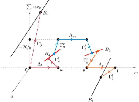
Fig. 1. An illustration of a singular connecting orbit projected to the space of (u, z1c1+

z2c2, w). Boundary layers atw= 0 andw= 1 exist if electroneutrality boundary conditions

are not assumed.

where prime is the derivative with respect to the fast variableξ=x/ε. Forε >0, the fast system (12) has the same phase portrait as that of slow system (11).

A singular (zeroth order in ε) orbit of the connecting problem will be a union of slow orbits (outer solutions) for theε= 0 limiting slow system and fast orbits (inner solutions) forε= 0 limiting fast system.

In view of the jumps of permanent charge Q(x) in (8) at x=a and x=b, the construction of singular orbits is split into three intervals [0, a], [a, b], [b,1] as follows. One preassigns six (unknown) values of (φ, c1, c2) atx=aandx=b:

φ(a) =φa, c1(a) =ca₁, c2(a) =ca₂; φ(b) =φb, c1(b) =cb₁, c2(a) =cb₂. (13)

Then these values determine two (boundary) sets atx=aandx=bas

Ba={(φa, u, ca₁, ca₂, J1, J2, a) : arbitraryu, J1, J2},

and

Bb={(φb, u, cb₁, cb₂, J1, J2, b) : arbitraryu, J1, J2}.

On each subinterval, a singular orbit can be constructed (see [12]) and typically consists of two singular (inner) layers and one regular (outer) layer (see Fig.1for an illustration).

(i) On interval [0, a], a singular orbit fromB0toBaconsists of two singular layers located at x= 0 and x=a, denoted as Γr₀ and Γl_a, and one regular layer Λl. Furthermore, with the preassigned values φa_,ca

1 and ca2, the flux Jkl andul(a) are uniquely determined so that

(ii) On interval [a, b], a singular orbit fromBa toBb consists of two singular layers located atx=aand x=b, denoted as Γr

a and Γlb, and one regular layer Λm. Furthermore, with the preassigned values (φa_{, c}a

1, ca2) and (φb, cb1, cb2, b), the flux Jm

k ,um(a) andum(b) are uniquely determined so that

(φa, um(a), ca1, c a 2, J

m 1 , J

m

2 , a)∈Ba and (φb, um(b), cb1, c b 2, J

m 1 , J

m

2 , b)∈Bb.

(iii) On interval [b,1], a singular orbit fromBb toB1 consists of two singular layers are located atx=bandx= 1, denoted as Γr

band Γl1, and one regular layer Λr. Furthermore, with the preassigned valuesφb_{, c}b

1 and cb2, the fluxJkr and ur(b) are uniquely determined so that

(φb, ur(b), cb1, c b 2, J

r 1, J

r

2, b)∈Bb.

The matching conditions for singular orbits of the full connecting problem are

J_kl =J_km=J_kr for k= 1,2, ul(a) =um(a) and um(b) =ur(b). (14)

The number of conditions in (14) is six, which is exactly the same number of unknowns preassigned in (13). In this way the singular connecting problem is reduced to the

governing system(14) (see [12] for an explicit form of the governing system).

Once a singular orbit is constructed and with some checkable transversality conditions, one can justify the validation of the singular orbit forε >0 small [12].

It should be pointed out that, typically, the internal layer Γa

l ∪Γamat x=ahas a conner at the joint so it is a double-layer (see Fig.1). Similarly, the internal layer Γb

m∪Γbr atx=bis also a double-layer.

We now recall the results on approximations of (φ, c1, c2, J1, J2) and µk’s from [46] for the case where z1 = 1 and z2 =−1 with L1 =L2 =L and R1 =R2 =R. We comment that, in [46], the electroneutrality boundary conditions L1 =L2 and R1=R2 are not required.

Based on the assumption thatQ0>0 is large,ε >0 is small and is smaller than 1/Q0, one can expand fluxes in εand inν= 1/Q0 nearε= 0 andν = 0.

First, one expands the fluxes inεas

J1(ε, ν) =J1(ν) +O(ε) and J2(ε, ν) =J2(ν) +O(ε),

where Jk(ν), depending also on the parameters (V, L, R, H(1), α, β), are the zeroth order inεterms of the fluxes. Then, one expandsJk(ν) aboutν as

J1(ν) =J10+J11ν+O(ν2) and J2(ν) =J20+J21ν+O(ν2).

Thus,

J1(ε, ν) =J10+J11ν+O(ν2, ε) and J2(ε, ν) =J20+J21ν+O(ν2, ε). (15)

The following result about the fluxes is established in [46].

Proposition 3.1. One has

J10= 0,

J11=

1 2H(1)(β−α)

(1−β)L+αR (1−β)√eV_L+α√_R

!2

(eVL−R);

J20= 2√LR

H(1)

1

(1−β)√L+α√e−V_R(

√

e−V_L−√_R),

J21=−

(β−α)eV_{LR (1−β)L+αR} H(1) (1−β)√eV_L+α√_R3(

√

e−V_L−√_R)

+ (e

V_{L−R) −V + lnL−lnR}

(1−β)L+αR3 4(β−α)H(1)(√e−V_L−√_{R) (1−β)}√_eV_L+α√_R3

− e

V_L−R 2(β−α)H(1)

(1−β)L+αR (1−β)√eV_L+α√_R

!2

. (16)

A distinct implication of J10= 0 in Proposition 3.1 is that large (positive) per-manent charge Q0 (or small ν = 1/Q0) inhibits the cation flux. We will provide a detailed discussion in Section 4 on what happens to the internal dynamics that is consistent with this conclusion.

To this end, we recall another immediate consequence of (16) (see [46] for more).

Corollary 3.2. [Current Saturation] For large permanent charge Q0 (small ν =

1/Q0) and to the leading order terms inν, individual fluxesJk’s, and hence, the total

current I saturate in |V|; more precisely, one has J20 is decreasing in V, concave

downward for V < V0∗ and concave upward for V > V0∗ for some V0∗, and J11 is

increasing in V, concave upward forV < V₁∗ and concave downward for V > V₁∗ for

someV1∗. Furthermore,|J20|and|J11|are uniformly bounded inV with a bound that

can be determined from the limits

lim

V→+∞J20=−

1 1−β

2R

H(1), V→−∞lim J20=

1 α

2L H(1),

lim

V→+∞J11=−V→lim+∞J21=

1 (1−β)2

((1−β)L+αR)2 2H(1)(β−α) ,

lim

V→−∞J11=−V→−∞lim J21=−

1 α2

((1−β)L+αR)2

2H(1)(β−α) . (17)

Proof. All the above statements can be derived from (16) easily.

Note that it is NOT the case if the permanent charge is small [23].

Remark 3.3. We want to emphasize that the formulas in (16) are established for boundedV. Strictly speaking, the formulas are not justified as|V| → ∞. The limits are presented, together with the monotone properties ofJ20andJ11in V, to allow the conclusion that, for boundedV,J20andJ11are bounded with a boundindependent

ofV.

presented a numerical study of the BVP with more or less the same setup as in our work: Dirichlet boundary conditions and the same form of the permanent charges, except that the nonzero value of the permanent charge, denoted there by −N (so that−N = 2Q0), was taken to be negative (N >0). In particular, the co-ion in [35] is the negatively charged ions and, in our case whereQ0>0, the co-ion is the cation (label with subscript 1). The boundary concentrations are special and fixed in [35] and are taken to be L=R= 1 (in terms of our notation). Numerical results were presented for relevant quantities asεvaries, asV varies, and asN varies.

It turns out our analytical results are consistent with the numerical results, say, reported in Figure 5.3.2 b, c of [35]. (We only examined the zeroth order terms inε so cannot compare with the numerical I–V curves with different ε values reported in Fig. 5.3.2a.) More precisely, our analytical results for the approximated currentI would be

I=J11ν−(J20+J21ν) up to O(ν2, ε),

and it can be checked from our formulas forJ20,J21 andJ11 withL=R= 1 fixed in the numerics in [35], that |I| is decreasing in N =−1/ν for fixed V, which is consistent with the qualitative behavior reported in Figure 5.3.2b.

Figure 5.3.2c in [35] reports numerical results for the co-ion (cation in our case) transport number τ1 =|J1|/|I| with the values N = 10, 20, 40. These values are moderate but could be viewed as large. In our case, for large Q0= 1/ν, the cation flux and anion flux are approximated as

J1=J10+J11ν+O(ν2, ε) =J11ν+O(ν2, ε), J2=J20+J21ν+O(ν2, ε).

Thus,

τ1=

|J1|

|I| =

|J11ν+O(ν2, ε)|

| −J20−J21ν+J11ν+O(ν2, ε)|

=|J11ν|

|J20|

+O(ν2, ).

Note also that, forL=R= 1 andh(x) = 1, one has, from (16),

J11= k1 (eV /2_{+ 1)}2(e

V _{−1) =} k1(e

V /2₋₁₎

eV /2_{+ 1} , J20=

k2(e−V /2−1) 1 +e−V /2 ,

where kj’s are constants results from α, β and H(1) in our formulas and are independent ofV. Thus, forV ≥0 but bounded,

τ1≈

|J11ν|

|J20| =k1

k2

(eV /2−1)(1 +e−V /2) (1−e−V /2_)(eV /2_{+ 1)}

2 N =

2k1 k2N ,

which is consistent with the numerical results presented in Figure 5.3.2c. The number τ1is nearly constant inV and, for fixedV, it decreases asNincreases. Also the trend in the figure indicates thatτ1 is close to zero asN becomes large.

4 Internal dynamics for

J

= 0

It follows from the Nernst–Planck equation in (9) that

J1 Z 1

0

1

Thus,J1has the same sign as that of ¯µ1(0)−µ¯1(1); in particular, if ¯µ1(0)−µ¯1(1)6= 0, thenJ16= 0.

For the setup of this paper, there are three regions of permanent charge Q(x): Q(x) = 0 for x∈[0, a)∪(b,1] and Q(x) = 2Q0 forx∈[a, b] withlargeQ0 orsmall ν= 1/Q0. A major consequence of largeQ0is, from Proposition3.1, up to the leading order inν= 1/Q0and inε, the flux of cation isJ10= 0, even if the transmembrane

potential µ¯1(0)−µ¯1(1)6= 0. We will reveal the internal dynamics that lead to this

conclusion. To do so, we will discuss what happens over each subinterval based on the approximated (zeroth order inε) profiles. Let

(φ(x;ε, ν), ck(x;ε, ν), Jk(ε, ν)) = (φ(x;ν), ck(x;ν), Jk(ν)) +O(ε) (18)

be the solution of the BVP (9) and (10). For ν > 0 small, one has the following expansions

J1(ν) =J10+J11ν+O(ν2),

whereJ10= 0 andJ11are given in (16). We will also provide figures for the profiles of rescaled electrical potentialφ(x;ν), cation concentrationc1(x;ν) and electrochemical potential ¯µ1(x;ν) of the cation, respectively. The parameter values used are

e0= 1.6022×10−19 (C), kB = 1.3806×10−23(J K−1), T = 273.16 (K),

V = 0.01 (V), L= 10 (M), R= 2×10−4(M), Q0= 2×103 (M), C0= 20 (M), a0= 0, b0= 25 (nm), A= (b0−a0)/3 (nm), B= (b0−a0)/2 (nm).

We comment that the value forQ0 is not physical. We use this value for some con-sistence of the size requirement of ε and Q0 in the key assumption given after the rescaling (7), which is required for a rigorous expansion used in this work. The com-parison of our analytic formulas to some numerical results in [35] at the end of the previous section indicates the analytical results could be valid for a more realistic range of the parameters. The corresponding dimensionless parameter values are

V = 0.425, L= 0.5, R= 10−5, a= 1 3, b=

1

2, ν = 10

−2_{, ε≈2×10}−3 ₍₁₉₎

The scaled cross-sectional areah(x) is taken to be

h(x) =  



π(−x+r0+a)2, x∈(0, a) πr₀2, x∈(a, b) π(x+r0−b)2, x∈(b,1).

The same choice of the parameter values will be used for figures in Section5. Notice that the whole interval is (0,1), and it is divided into three subintervals (0, a),(a, b) and (b,1). Permanent charge is located over (a, b). The radius of the neck of ion channel isr0. In the figures, we letr0= 0.5.

4.1 Internal dynamics over the interval(0, a)

The leading order terms of (φ, c1,µ¯1) in (18) are derived in [46]. One has

Proposition 4.1. Forx∈(0, a),

where

c10(x) =L−J20

2 H(x), φ0(x) =V −ln c10(x)

L , ¯

µ10(x) =φ0(x) + lnc10(x) =V + lnL.

The following direct consequence explains the reason forJ10= 0 over (0, a).

Corollary 4.2. Over the interval (0, a),c10(x) =O(1) but µ¯0₁₀(x) = 0, and hence,

one hasJ10= 0.

4.2 Internal dynamics over the interval(a, b)

It follows again from [46] that one has the following approximations.

Proposition 4.3. Forx∈(a, b),

φ(x;ν) = −lnν+φ0(x) +O(ν), c1(x;ν) =c10(x) +c11(x)ν+O(ν2), ¯

µ1(x;ν) = ¯µ10(x) +O(ν),

where

φ0(x) = ln2e V_L

A2 0

, c10(x) = 0, c11(x) =1 2A

2

0−J11(H(x)−H(a)),

¯

µ10(x) =φ0(x) + lnc11(x) = ln _H(b)

−H(x) H(b)−H(a)e

V_L+H(x)−H(a) H(b)−H(a)R

with

A0=

√

eV_{L((1−β)L+αR)} (1−β)√eV_L+α√_R .

Note that the expansion of φ(x;ν) in ν is not regular with the term −lnν over this interval and the zeroth order term ¯µ10(x) involves the first order term c11(x).

One has the following immediate consequence providing a mechanism forJ10= 0 over (a, b) that is different from that over (0, a).

Corollary 4.4.Over the interval(a, b),c10(x) = 0, and hence,J10= 0. Furthermore, ¯

µ10(a) =V + lnL and µ¯10(b) = lnR, and, as R decreases, µ¯10(a)−µ¯10(b) =V +

lnL−lnR increases (without an upper bound independent of R).

Proof. It follows from Proposition4.3directly.

4.3 Internal dynamics over the interval(b,1)

Proposition 4.5. Forx∈(b,1),

where

c10(x) =R+ J20

2 (H(1)−H(x)), φ0(x) = lnR−lnc10(x), ¯

µ10(x) =φ0(x) + lnc10(x) = lnR.

The following consequence shows a mechanism for J10 = 0 over (b,1) that is similar to that over (0, a).

Corollary 4.6. Over the interval (b,1), c10(x) =O(1) andµ¯010(x) = 0, and hence, J10= 0.

4.4 Summary of mechanism for J10= 0

From the above discussion, we conclude that the mechanisms forJ10= 0 are different over each subintervals. More precisely, one has,

– over the first interval (0, a), J10= 0 is the result of constant µ¯10(x) = ¯µ10(0) (so that ¯µ0₁₀(x) = 0) whilec10(x)6= 0;

– over the last interval (b,1),J10= 0 is the result ofconstantµ¯10(x) = ¯µ10(1) (so that ¯µ0

10(x) = 0) whilec10(x)6= 0;

– over the interval (a, b) where permanent charge is large,J10= 0 is the result of c10(x) = 0 while ¯µ10(x) is not a constant, in particular, the drop of ¯µ10(x) over (a, b) equals its drop over (0,1), in fact, ¯µ10(a) = ¯µ1(0) and ¯µ10(b) = ¯µ1(1).

Here we provide the profiles of concentrationc1(x;ν) (Fig.2), electrical potential φ(x;ν) (Fig.3) and electrochemical potential ¯µ1(x;ν) (Fig.4) over the whole interval [0,1]. The concentrationc1(x;ν) and the electrical potentialφ(x;ν) are not continuous atx=a= 1/3 andx=b= 1/2 due to the discontinuity of the permanent charge at these point. On the other hand, the electrochemical potential ¯µ1(x;ν) is continuous.

5 Declining phenomenon and internal dynamics

In this section, we will show that large permanent charge is a mechanism for the

declining phenomenon described in the introduction. Recall that, by the declining

phenomenon, we mean the following:

For fixedV andL, asRdecreases, the flux of counterion (J2 in the setting since

Q0>0) decreases monotonically without a positive lower bound.

Remark 5.1. The phenomenon was well-known in the physiology community. Unfor-tunately, we could not find references stating precisely this phenomenon. We have contacted many leading experts who are all recognizing this phenomenon. Some experts mention this phenomena as an example of ‘exchange diffusion’ and/or long channel phenomena.

0 0.2 0.4 0.6 0.8 1 −0.1

0 0.1 0.2 0.3 0.4 0.5 0.6

Concentration of Cation in (0,1)

x

c1(x)

Fig. 2.Profile ofc1(x;ν) over [0,1]. Note thatc10(x) = 0 forx∈(a, b) and, forR= 10−5

small chosen for the numerics and sinceJ20=O(

√

R),c10(x)≈L= 0.5 for x∈(0, a) and

c10(x) =O(

√

R) is close to zero forx∈(b,1).

0 0.2 0.4 0.6 0.8 1

−6 −4 −2 0 2 4 6 8

Electropotential in (0,1)

x

phi(x)

Fig. 3. Profile of φ(x;ν) over [0,1]: For ν = 10−2 _{and R = 10}−5 _{small chosen for the}

0 0.2 0.4 0.6 0.8 1 −12

−10 −8 −6 −4 −2 0

Electrochemical Potential of Cation in (0,1)

x

mu1(x)

Fig. 4. Profile of ¯µ1(x;ν) over [0,1]. For ν = 10−2 and R = 10−5 small chosen for the

numerics, ¯µ1(x;ν)≈V + lnL=−0.214 forx∈(0, a) and ¯µ1(x;ν)≈lnR=−11.5 forx∈

(b,1). Note the large drop of ¯µ1 over the interval (a, b) = (1/3,1/2) and the nearly constant

values over the other two subintervals.

5.1 Experimental phenomena are consistent with our analysis

The formula for J20 in (16) actually justifies the declining phenomenon, up to the leading orderJ20in ν for smallν (or for largeQ0); that is,

Proposition 5.2. As a function of R, the leading order term J20 of the flux is

monotonically decreasing and concave downward. Furthermore, as R deceases, |J20|

deceases (without lower bound independent of R).

Proof. Indeed, from the expression ofJ20in (16) and treatingJ20as a function ofw

whereR=w2for convenience, one has

J20(w) =

√

L 2H(1)

√

e−V_Lw−w2 (1−β)√L+α

√

e−V_w.

It is clear thatJ20(w)→0+_{as w→0}+_{. Note that the derivative ofJ}

20in wis

J₂₀0 (w) = 1 2H(1)

(1−β)L√e−V _−2(1−β)√_Lw−α√_e−V_w2 [(1−β)√L+α√e−V_w]2 .

Thus, from the expression of the numerator, if w is smaller than some w0, then J₂₀0 (w)>0, and hence, as w→0+ _{(or equivalently,R→0) monotonically over the} interval [0, w0],J20(w)→0 monotonically.

1 0.9 0.8 0.7 0.6 0.5 0.4 0.3 0.2 0.1 0

R 10-3

0 1 2 3 4 5 6

j20

10-11 The zero-th order of Flux of Anion

Fig. 5. Declining curve:J20vsRforR∈(0,10−3] withL= 0.5 andV = 0.425.

In Figure 5, the horizontal axis is for R and the vertical for J20. We fix V = 0.425 and L= 0.5 as in (19), and vary R∈(0,10−3_{]. The monotonicity and concave} downward features of the graph are apparent.

Remark 5.3. We comment that, for large permanent charge, the declining curve phenomenon occurs when the transmembrane electrochemical potential ¯µ2(0)−µ¯2(1) is increasingin a particular way; that is, as R deceases with fixed V and L. If one increases the transmembrane electrochemical potential ¯µ2(0)−µ¯2(1) in a different manner, for example, as|V|increases or asLincreases, Corollary3.2shows that the declining curve phenomenon does not happen.

It is also important to note that, when the next order term J21ν is considered, then, as R decreases, |J21| increases. But, if R and νlnR are small, then |J21ν| stays small. Thus, only whenν is very small (Q0is very large), is the termJ21ν not significant, and hence, the termJ20dominates the described behavior.

5.2 Mechanism of declining phenomena from the profiles

Recall, from the Nernst–Planck equation in (9) that

−J2=D2(x)h(x)c2(x;ν) d

SinceD2(x) andh(x) are fixed, we will treat them as of orderO(1) quantities so that they do not contribute much to the near zero flux scenario whenRis small. Thus, as far as the near zero flux mechanism is concerned, one has

−J2≈c2(x;ν)¯µ02(x;ν). (20)

One sees that the gradient ¯µ0

2(x;ν) of the electrochemical potential is the main driving force for the flux J2. Intuitively, large drop of (or transmembrane) electro-chemical potential ¯µ2(0)−µ¯2(1) of ¯µ2 produces large flux J2. In this sense, the declining curve phenomenon is rather counterintuitive. A careful look at (20) reveals that there is only one possibility for the declining curve phenomenon; that is, when-ever ¯µ02(x;ν) is large,c2(x;ν) has to be much smaller in order to produce a small flux

|J2|. We will apply the analytical results of the internal dynamics from [46] to show that this is indeed the case.

For fixed V and L, ¯µ2(0)−µ¯2(1) =−V + lnL−lnR≈ −lnR1 for small R. We need to understand

(i) HOW the electrochemical potential ¯µ2 drops an orderO(−lnR)1 over the intervalx∈[0,1];

(ii) HOWJ2 can be small, for smallν andR, at everyx∈[0.1];

(iii) Most importantly, HOW the above two things, with the constraint (20), can happen simultaneously.

There are two small parametersν andRin this consideration. The relative sizes of these two parameters is relevant for J20 being a good approximation for J2. It turns out we will needνlnR1. In order to show this, we will examine the profiles of (φ(x;ν), c2(x;ν),µ¯2(x;ν)) up to orderO(ν).

We now discuss what happens over each subinterval based on the approximated (of zeroth order inε) functions of profiles. To do so, let

(φ(x;ε, ν), c2(x;ε, ν), J2(ε, ν)) = (φ(x;ν), c2(x;ν), J2(ν)) +O(ε)

be the solution of the boundary value problem. Forν >0 small, one has the following expansions

J2(ν) =J20+J21ν+O(ν2),

whereJ20 andJ21are given in (16). The expansions inν forφ(x;ν) andc2(x;ν) are

notregularover (a, b) and are qualitatively different over the subintervals (0, a), (a, b)

and (b,1). They will be given explicitly in each subsection below for us to understand what happens over each subinterval.

5.2.1 Internal dynamics over the interval(0, a)

The leading order terms of (φ, c2) are derived in [46]. One has

Proposition 5.4. Forx∈(0, a),

0 0.05 0.1 0.15 0.2 0.25 0.3 0.35 0.494 0.495 0.496 0.497 0.498 0.499 0.5 0.501

Concentration of Anion in (0,a)

x

c2(x)

0 0.05 0.1 0.15 0.2 0.25 0.3 0.35

0.425 0.4255 0.426 0.4265 0.427 0.4275 0.428 0.4285

Electropotential in (0,a)

x

0 0.05 0.1 0.15 0.2 0.25 0.3 0.35

−1.1275 −1.127 −1.1265 −1.126 −1.1255 −1.125 −1.1245

Electrochemical Potential of Anion in (0,a)

x

mu2(x)

Fig. 6. Profiles of c2(x;ν), φ(x;ν), and ¯µ2(x;ν) over interval [0, a]. For ν = 10−2 and

R= 10−5 small used for numerics, c2(x;ν) =L+O(

√

R)≈0.5,φ(x;ν) =V +O(√R)≈ 0.43, and ¯µ2(x;ν)≈ −V + lnL=−1.12.

where

φ0(x) =V −lnc20(x)

L , φ1(x) =− c21(x) c20(x)

+2J11 J20

lnc20(x) L ;

c20(x) =L− J20

2 H(x), c21(x) =−

J11+J21 2 H(x);

In particular,µ¯2(x;ν) = ¯µ20(x) + ¯µ21(x)ν+O(ν2), where

¯

µ20(x) =−V + 2 lnc20(x)−lnL, µ¯21(x) = 2 _c

21(x) c20(x)−

J11 J20

lnc20(x) L

.

Note thatc20(x) =c10(x) andc21(x) =c11(x) forx∈(0, a).

Figure6 shows profiles ofc2(x;ν),φ(x;ν) and ¯µ2(x;ν) over the interval (0, a).

Corollary 5.5. Over the interval(0, a),c2(x;ν) =O(1)but

¯

µ0₂(x;ν) =− J20

h(x)c20(x)+O(νlnR) =O(

√

R, νlnR).

Therefore, from (20),

J2≈c2(x;ν) d

dxµ¯2(x;ν) =O(1)O(

√

andµ¯2(x;ν)drops an order ofO(√R, νlnR)over the interval(0, a).

In particular, for zeroth order in ν,J20=O(

√

R)andµ¯0₂₀(x) =O(√R)over the interval (0, a).

5.2.2 Internal dynamics over the interval(a, b)

It follows from [46] that

Proposition 5.6. Forx∈(a, b),

φ(x;ν) =−lnν+φ0(x) +φ1(x)ν+O(ν2),

c2(x;ν) =2 ν +

1 2A

2

0−J11(H(x)−H(a))

ν+O(ν2),

whereA0 is given in Proposition 4.3, and

φ0(x) = ln2e V_L

A2 0

, φ1(x) =φa₁−A0+ J20

2 (H(x)−H(a)),

A1=

α(β−α)eVLR((1−β)L+αR) 2 (1−β)√eV_L+α√_R3

√

e−V_L−√_R

+ α(V −lnL+ lnR)((1−β)L+αR)

3 _eV_L−R 8(β−α)(√e−V_L−√_{R) (1−β)}√_eV_L+α√_R3,

φa₁ =ln A2

0

eV_LR

ln L eV_R

β−α

α (L−A0)−2

(1−β)√eV_L+α√_R α√R

A1 A0

+ 2(1−β)

√

eV_L

α√R A1 A0

−β

α(L−A0) +L.

In particular,µ¯2(x;ν) = ¯µ20(x) + ¯µ21(x)ν+O(ν2_)where

¯

µ20(x) =−φ0(x) + ln 2 = ln A 2 0

eV_L, µ¯21(x) =−φ a

1+A0− J20

2 (H(x)−H(a)). The profiles of c2(x;ν),φ(x;ν), and ¯µ2(x;ν) are shown in Figure7.

Note that, over this interval, bothφ(x;ν) andc2(x;ν) aresingularinν. To under-stand what happens to the internal dynamics for anions over the interval (a, b), we need to resolve this singularity by considering at leastO(ν)-terms.

Corollary 5.7. Over the interval (a, b), c2(x;ν) = O(1/ν) 1 and µ¯2(x;ν) = O(lnR)1 but

¯

µ0₂(x;ν)≈µ¯0₂₁(x)ν =− J20

2h(x)ν=O(ν

√

R).

Therefore, from (20),

J2≈O(1/ν)O(ν

√

R) =O(√R) and µ¯2(x;ν) only drops O(ν√R) over (a, b).

0.32 0.34 0.36 0.38 0.4 0.42 0.44 0.46 0.48 0.5 200

200.0002 200.0004 200.0006 200.0008 200.001 200.0012 200.0014

Concentration of Anion in (a,b)

x

c2(x)

0.32 0.34 0.36 0.38 0.4 0.42 0.44 0.46 0.48 0.5

6.4348 6.4348 6.4348 6.4348

Electropotential in (a,b)

x

phi(x)

0.32 0.34 0.36 0.38 0.4 0.42 0.44 0.46 0.48 0.5

−1.1365 −1.1365 −1.1365 −1.1365 −1.1365 −1.1365 −1.1365 −1.1365

Electrochemical Potential of Anion in (a,b)

x

mu2(x)

Fig. 7. Profiles of c2(x;ν), φ(x;ν), and ¯µ2(x;ν) over interval [a, b]. For ν = 10−2 and

R= 10−5 _{small used for numerics,c}

2(x;ν) = 2/ν+O(ν)≈200,φ(x;ν) =−lnν+φ0(x) +

O(ν)≈6.0, and ¯µ2(x;ν) =−φ0(x) + ln 2≈ −1.10.

to the total drop ¯µ2(0)−µ¯2(1) =O(−lnR)1 for smallR. The only way to realize the large total drop ¯µ2(0)−µ¯2(1) is that ¯µ2(x;ν) dropsO(−lnR) over the subinterval (b,1). Indeed, this is the case as shown below.

5.2.3 Internal dynamics over the interval(b,1)

Proposition 5.9. Forx∈(b,1),

φ(x;ν) =φ0(x) +φ1(x)ν+O(ν2), c2(x;ν) =c20(x) +c21(x)ν+O(ν2),

where

φ0(x) = −lnc20(x)

R , φ1(x) =− c21(x) c20(x)+

2J11 J20

lnc20(x) R ;

c20(x) =R+J20

2 (H(1)−H(x)), c21(x) =

J11+J21

2 (H(1)−H(x));

In particular,µ¯2(x;ν) = ¯µ20(x) + ¯µ21(x)ν+O(ν2)where

¯

µ20(x) = 2 lnc20(x)−lnR, µ¯21(x) =2c21(x) c20(x) −

2J11 J20

0.5 0.6 0.7 0.8 0.9 1 0

1 2 3 4 5 6 7x 10

−3 _{Concentration of Anion in (b,1)}

x

c2(x)

0.5 0.6 0.7 0.8 0.9 1

−6 −5 −4 −3 −2 −1 0

Electropotential in (b,1)

x

phi(x)

0.5 0.6 0.7 0.8 0.9 1

−12 −10 −8 −6 −4 −2 0

Electrochemical Potential of Anion in (b,1)

x

mu2(x)

Fig. 8. Profiles of c2(x;ν), φ(x;ν), and ¯µ2(x;ν) over interval [b,1]. For ν = 10−2 and

R= 10−5 small used for numerics, c2(x;ν) =O(

√

R, ν), φ(x;ν) =φ0(x) +O(ν)≈ −5.0,

and ¯µ2(b;ν)≈ −1.10 and ¯µ2(1) = lnR≈ −11.5.

The profiles of c2(x;ν),φ(x;ν), and ¯µ2(x;ν) over (b,1) are shown in Figure8.

Corollary 5.10. Over the interval (b,1), for small ν and R, c20(x) changes from

c20(b) =O(√R) toc20(1) =R monotonically, and µ¯2(x;ν) changes from µ¯2(b;ν) = O(1)toµ¯2(1) = lnR. Therefore, forx∈(b,1), from (20),

J2≈O(

√

R) and µ¯2(x;ν) drops O(−lnR) over (b,1).

Remark 5.11. Note that, over this interval, the order of ¯µ02(x;ν) varies inxfrom ¯

µ0₂(b;ν) =O(1) to ¯µ0₂(1;ν) =O(1/√R) but overall drops isO(−lnR). This is different from what happened over the intervals (0, a) and (a, b).

5.3 Summary of mechanism for declining phenomenon

In summary, for smallν andR, with the technical assumption thatνlnR≤√R, we have,J2=O(

√

0 0.2 0.4 0.6 0.8 1 0

50 100 150 200 250

Concentration of Anion in (0,1)

x

c2(x)

Fig. 9.Profilec2(x;ν) over [0,1].

(i) over (0, a), one has c2(x;ν) = O(1) but ¯µ0₂(x;ν) =O(√R)1 so that J2 =

O(√R); (Note that the drop of µ¯2 over the interval (0, a) is of order O(

√

R),

which has nearly no contribution to the drop ofµ¯2over the whole interval(0,1).)

(ii) over (a, b), c2(x;ν) =O(1/ν) but ¯µ02(x;ν) = O(ν

√

R) so that J2 =O(

√

R);

(Note that the drop ofµ¯2 over the interval (a, b)is of orderO(ν

√

R), which is

even smaller than that over the subinterval (0, a)and, of course, has nearly no

contribution to the drop ofµ¯2 over the whole interval(0,1).)

(iii) over (b,1), different from what happened over each of the previous two subin-tervals, the orders of c2(x;ν) and ¯µ0₂(x;ν) are NOT uniform forx∈(b,1) but the drop of O(lnR) in ¯µ2(x;ν) is fully realized over this subinterval (b,1) (see Remark5.11).

We comment that, for large Q0>0, when R is small, both the transmembrane electrochemical potentials ¯µ1(0)−µ¯1(1) =V+ lnL−lnRfor the cation and ¯µ2(0)− ¯

µ2(1) =−V + lnL−lnR for the anion are large. The drop of ¯µ1(x;ν) is mainly realized over the interval (a, b) but the drop of ¯µ2(x;ν) is mainly realized over the interval (b,1).

0 0.2 0.4 0.6 0.8 1 −6

−4 −2 0 2 4 6 8

Electropotential in (0,1)

x

phi(x)

Fig. 10.Profile ofφ(x;ν) over [0,1].

0 0.2 0.4 0.6 0.8 1

−12 −10 −8 −6 −4 −2 0

Electrochemical Potential of Anion in (0,1)

x

mu2(x)

Fig. 11.Profile of ¯µ2(x;ν) over [0,1].

6 Concluding remarks

that one of the defining properties of transporters, obligatory exchange, can arise in an open channel with just one structure. When the permanent charge is large, the current carried by counter ions, majority charge carriers with the opposite sign from the permanent charge, can decline, even to zero, as the driving force (the gradient of electrochemical potential) increases. We also show that large permanent charges essentially inhibit the flux of co-ions, regardless of the magnitude of transmembrane electrochemical potential.

We thank the anonymous referees for their comments, particularly, one of the referees for his/her invaluable remarks and suggestions on the mathematical treatments of expansions in two small parameters that help improve the manuscript.

It is a pleasure to thank Mordy Blaustein, Don Hilgemann and Ernie Wright for help with the literature of transporters and Chris Miller for help with the original formulation of the declining phenomenon in Section5. LZ thanks the University of Kansas for its hospitality during her visit from October 2016 to October 2017 when this research is conducted. LZ is partially supported by NNSF of China grants no. 11431008 and no. 11771282, and the Joint Ph.D. Training Program sponsored by the Chinese Scholarship Council.

References

1. J.N. Abelson, M.I. Simon, S.V. Ambudkar, M.M. Gottesman, ABC Transporters: Biochemical, Cellular, and Molecular Aspects(Academic Press, 1998)

2. P.F. Baker, M.P. Blaustein, A.L. Hodgkin, R.A. Steinhardt, J. Physiol.200, 431 (1969) 3. M.P. Blaustein, W.J. Lederer, Physiol. Rev.79, 763 (1999)

4. P. Chlanda, E. Mekhedov, H. Waters, C.L. Schwartz, E.R. Fischer, R.J. Ryham, F.S. Cohen, P.S. Blank, J. Zimmerberg, Nat. Microbiol.1, 16050 (2016)

5. B. Eisenberg, W. Liu, Mol. Based Math. Biol.5, 125 (2017) 6. B. Eisenberg, ASBMB Today13, 36 (2014)

7. B. Eisenberg, Fluct. Noise Lett.11, 1240001 (2012)

8. B. Eisenberg, Crowded charges in ion channels, inAdvances in Chemical Physics, edited by S.A. Rice, A.R. Dinner (John Wiley & Sons, Inc., 2012), Vol. 148, pp. 77–223 9. R.S. Eisenberg, J. Memb. Biol.150, 1 (1996)

10. R.S. Eisenberg, Atomic biology, electrostatics and ionic channels, inNew Developments and Theoretical Studies of Proteins, edited by R. Elber (World Scientific, Philadelphia, 1996), pp. 269–357

11. R.S. Eisenberg, J. Memb. Biol.115, 1 (1990)

12. B. Eisenberg, W. Liu, SIAM J. Math. Anal.38, 1932 (2007) 13. B. Eisenberg, W. Liu, H. Xu, Nonlinearity28, 103 (2015) 14. O. Frohlich, R.B. Gunn, Biochem. Biophys. Acta864, 169 (1986)

15. D. Gillespie, A singular perturbation analysis of the Poisson–Nernst–Planck system: Applications to Ionic Channels, Ph.D. Dissertation, Rush University at Chicago, 1999 16. J. Griffiths, C. Sansom,The Transporter Facts Book(Academic Press, 1997)

17. F. Helfferich,Ion Exchange(1995 Reprint) (McGraw Hill reprinted by Dover, 1962) 18. B. Hille,Ion Channels of Excitable Membranes, 3rd edn. (Sinauer Associates Inc., 2001) 19. B. Hille, Transport Across Cell Membranes: Carrier Mechanisms, in Textbook of Physiology, edited by H.D. Patton et al. (Saunders, 1989), Vol. 1, Chap. 2, pp. 24–47 20. A.L. Hodgkin, Biol. Rev.26, 339 (1951)

21. S. Ji, B. Eisenberg, W. Liu, J. Dyn. Differ. Equ. (2017), https://doi.org/10.1007/ s10884-017-9607-1

22. S. Ji, W. Liu, J. Dyn. Differ. Equ.24, 955 (2012)

23. S. Ji, W. Liu, M. Zhang, SIAM J. Appl. Math.75, 114 (2015) 24. R.D. Keynes, R.C. Swan, J. Physiol.147, 591 (1959)

27. W. Liu, J. Differ. Equ.246, 428 (2009)

28. W. Liu, B. Wang, J. Dyn. Differ. Equ.22, 413 (2010) 29. W. Liu, X. Tu, M. Zhang, J. Dyn. Differ. Equ.24, 985 (2012) 30. W. Liu, H. Xu, J. Differ. Equ.258, 1192 (2015)

31. M. Lu, J. Symersky, M. Radchenko, A. Koide, Y. Guo, R. Nie, S. Koide, Proc. Natl. Acad. Sci. U. S. A.110, 2099 (2013)

32. H. Miedema, M. Vrouenraets, J. Wierenga, W. Meijberg, G. Robillard, B. Eisenberg, Nano Lett.7, 2886 (2007)

33. W. Nonner, R.S. Eisenberg, Biophys. J.75, 1287 (1998)

34. R.F. Pierret,Semiconductor Device Fundamentals(Addison Wesley, 1996)

35. I. Rubinstein, Electro-Diffusion of Ions, inSIAM Studies in Applied Mathematics(SIAM, Philadelphia, PA, 1990), Vol. 11

36. B. Sakmann, E. Neher,Single Channel Recording, 2nd edn. (Plenum, 1995)

37. W.D. Stein, T. Litman,Channels, carriers, and pumps: an introduction to membrane transport(Elsevier, 2014)

38. R.B. Stockbridge, L. Kolmakova-Partensky, T. Shane, A. Koide, A. Koide, C. Miller, S. Newstead, Nature525, 548 (2015)

39. S.M. Sze,Physics of Semiconductor Devices(John Wiley & Sons, 1981) 40. F.L. Theodoulou, I.D. Kerr, Biochem. Soc. Trans.43, 1033 (2015)

41. D. Tosteson, Membrane Transport: People and Ideas(American Physiological Society, 1989)

42. H.H. Ussing, Acta Physiolog. Scand.19, 43 (1949) 43. H.H. Ussing, Nature160, 262 (1947)

44. D. Vasileska, S.M. Goodnick, G. Klimeck, inComputational Electronics: Semiclassical and Quantum Device Modeling and Simulation(CRC Press, 2010), Vol. 764

45. W. Wang, R. MacKinnon, Cell169, 422 (2017)

46. L. Zhang, W. Liu, Poisson–Nernst–Planck systems for ion channels with large permanent charges. Preprint.