Q Deformation in Gaussian Map

Q-Deformation in Gaussian Map

1

Applied Physics Department, Priyadarshini J L College of Engineering

Abstract: Q-deformed Gaussian map is presented in the following text. A general introduction to nonlinear maps is given. Quantum group which leads to the q-deformation process of nonlinear dynamical system is touched upon. A brief introduction of q-deformed number is given.

Keywords: Q-deformation, Quantum groups, Nonlinear maps, Hopf algebra, X-space.

I. INTRODUCTION

Maps in nonlinear dynamical systems are known variously as difference equations, recursion relations, iterated maps, or simply maps. For instance, suppose we repeatedly pressed the cosine button on the calculator, starting from some number . Then the successive readouts are = cos , = cos and so on.[1] Set your calculator to radian mode and try it. Can you explain the surprising result that emerges after many iterations? The rule = cos , is an example of a one-dimensional map, so-called because the points belong to the one-dimensional space of real numbers. The sequence , , , … …. is called the orbit starting from . Maps arise in various ways:

A. As tools for analyzing differential equations. We have already encountered maps in this role. For instance, Poincare’ maps allowed us to prove the existence of a periodic solution for the driven pendulum and Josephson junction, and to analyze the stability of periodic solutions in general. The Lorenz map provided strong evidence that the Lorenz attractor is truly strange, and is not just a long-period limit cycle.

B. As models of natural phenomena. In some scientific contexts it is natural to regard time as discrete. This is the case in digital electronics, in parts of economics and finance theory, in impulsively driven mechanical systems, and in the study of certain animal populations where successive generations do not overlap.

C. As simple examples of chaos. Maps are interesting to study in their own right, as mathematical laboratories for chaos. Indeed, maps are capable of much wilder behavior than differential equations because the points hop along their orbits rather than flow continuously.

II. QUANTUMGROUPSASPRECURSORTO Q-DEFORMATION

There is an emergence in the studies of quantum group recently leading to analysis of several q-deformed physical systems. Theory of quantum groups turned the attention of physicists to the rich mathematics of q-series, q-special functions, etc., with a history going back to the nineteenth century [2]. Here we suggest a scheme of q-deformation of nonlinear maps. We will explain the mechanism of q-deformation using nonlinear maps.

But first let’s take look at quantum groups in brief. A quantum group is a kind of non-commutative algebra with additional structures. In general, a quantum group is some kind of Hopf algebra [3]. There is no single, all-encompassing definition, but instead a family of broadly similar objects. Let G be a group in the usual sense, i. e. a set satisfying the group axioms, and k be a field. With this group one can associate a commutative, associative k-algebra of functions from G to k with point wise algebra structure, i. e. for any two elements f and f’, for any scalar ∈ and ∈ we have,

( + )( )≔ ( ) + ( )

( )( )≔ ( )

( )( )≔ ( ) ′( )

ClassicalgroupG Axiomsofagroup →

Commutativealgebraof functionsonGwith correspondingextraaxioms

Quantumgroup (Abstractobject) ↔

Non−commutativealgebrawithsame extraaxioms; "algebraof functionsonaquantumgroup"

There is a similar concept of “quantum spaces”: If G acts on a set X (e. g. a vector space), there is a corresponding so-called

coaction of the commutative algebra of functions on G on the commutative algebra of functions on X satisfying certain axioms. The latter algebra can often be deformed/quantized into a non-commutative algebra, called the “algebra of functions on a quantum space” with a similar coaction. There are three ways of considering algebras of functions on a group and their deformations:

Polynomial functions Poly(G) (developed by Woronowicz and Drinfel’d)

Continuous functions C(G), if G is a topological group (developed by Woronowicz) Formal power series (developed by Drinfel’d)

The notion of deformation is not uncommon in physics. Quantum mechanics may be viewed as a deformation of classical mechanics, the deformation parameter being h. Relativistic kinematics can be looked upon as deformation of Newtonian kinematics. Here, f3 = v/c plays the role of deformation parameter. In a similar vein, quantum algebras are nonlinear extension of classical Lie algebras i.e. in general, the commutators between generators are no longer a linear combination of the generators of the set. These algebras contain one or more deformation parameters, such that in the appropriate limit of these parameters, quantum algebras go back to classical Lie algebras. The word ‘quantum’ was initially used to denote these algebras owing to analogy with the above mentioned limiting relation between classical and quantum mechanics. The relation between quantum groups and their algebras is much like the same, as between Lie groups and Lie algebras. Thus a quantum algebra is generated by infinitesimal generators of the corresponding quantum group. In case of a classical Lie group, its elements can be obtained by an exponential map from the Lie algebra generators with a set of abelian group parameters. Whereas, in case of quantum groups, we have a similar relationship between quantum group and quantum algebra, only that the group parameters become non-commuting among themselves. This situation is similar to the commuting variables of classical mechanics becoming operators in quantum mechanics. The concept of a quantum algebra (or quantum group) goes back to late seventies. It was introduced independently, by Kulish and Reshitikhin, Sklyanin, Drinfeld and Jimbo under different names, like quantized universal enveloping algebras or (Hopf algebras) and independently by Woronowicz in terms of compact matrix pseudogroup. In the approach of Manin, quantum algebras are identified with linear transformations on quantum planes with non-commutative coordinates. Wess and Zumino developed the differential calculus on non-commutative planes. In the following, we describe briefly the alternative approaches due to Manin to quantum groups. For the connections between different approaches, the reader is referred to literature.

III.WHATISQ-DEFORMATION

In 1846 Heine [4] defined a number to a basic number as,

[ ] = (1)

Such that [ ] →n when q →1. In 1904 Jackson defined a q-exponential function given by

=∑

= (6)

Which also has the property that in the limit q →1, [ ] → . The associated q-exponential function is given by equation (2) but with [ ] defined according to (5).

In non-extensive statistical mechanics of Tsallis [4], a new q-exponential function has been introduced as,

= (1 + (1− ) )/( ) ₍₇₎

Which satisfies the nonlinear equation given by,

( )

= ( ( )) (8)

And has the required limiting behavior: →exp( ) when →1. This plays a very important role in the non-extensive statistical mechanics by replacing exp( ) in certain domains of application. It should be noted that it is natural to define a generalized exponential function as in (6) if we consider the relation,

= lim → 1 + (9)

And regard 1/N as a continuous parameter. The non-extensive statistical mechanics has found applications in a wide range of physical problems [6], including the study of nonlinear maps at the edge of chaos.

IV.Q-DEFORMATIONINGAUSSIANMAP

Here we will give the example of Gaussian map which is based on the Gaussian exponential function. It is characterized by two parameters b and c as follows,

= + (Gaussian map) (10)

The q-deformed version of Gaussian map i.e. q-Gaussian map of the above definition of the q-deformation of one-dimensional nonlinear map is given as,

= {[ ] } _{+ (q-Gaussian map) (11)}

Or, = ( )( ) _{+ (q-Gaussian map) (12)}

Which is under the limit →1 becomes the original Gaussian map.

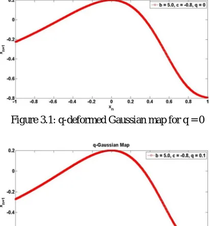
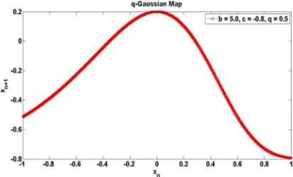
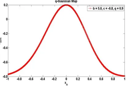
Let’s see how this happens with plots for different values of q for q-Gaussian map shown below. The successive plots of q-Gaussian map are plotted for = 0 to = 1.

Figure 3.1: q-deformed Gaussian map for q = 0

Figure 3.3: q-deformed Gaussian map for q = 0.2

Figure 3.4: q-deformed Gaussian map for q = 0.3

Figure 3.7: q-deformed Gaussian map for q = 0.6

Figure 3.8: q-deformed Gaussian map for q = 0.7

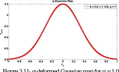
Figure 3.9: q-deformed Gaussian map for q = 0.8

Figure 3.11: q-deformed Gaussian map for q = 1.0

V. CONCLUSIONS

We have discussed the q-deformed Gaussian map. The q-deformation of Gaussian map is espoused by plotting the maps in MATLAB with changing the q-deformation parameter from 0 to 1. It shows that as the parameter q approaches 1, the original map is recovered. The q-deformation of nonlinear maps find applications in a number of areas, including the study of fractals and multi-fractal measures, and expressions for the entropy of chaotic dynamical systems. The relationship to multi-fractals and dynamical systems results from the fact that many fractal patterns have the symmetries of Fuchsian groups in general and the modular group in particular. The connection passes through hyperbolic geometry and ergodic theory, where the elliptic integrals and modular forms play a prominent role. One more advantage with the study of q-deformed nonlinear maps is that the additionally introduced deformation parameter can be varied as per our requirements to fit a possible large range of functional forms, which are similar in nature.

REFERENCES

[1] Strogatz, S. H. (2014). Nonlinear dynamics and chaos: with applications to physics, biology, chemistry, and engineering. Westview press [2] Gasper, G., & Rahman, M. (1990). Basic hypergeometric series, volume 35 of Encyclopedia of Mathematics and its Applications [3] Podleś, P., & Müller, E. (1998). Introduction to quantum groups. Reviews in Mathematical Physics, 10(04), 511-551.

[4] E. Heine, “Handbuch der Kuqelfunktionen’, 1, Reimer, Berlin(1878), reprinted by Physica-Verlag, Wurzburg (1961).

[5] Tsallis, C. (1999). Nonextensive statistics: theoretical, experimental and computational evidences and connections. Brazilian Journal of Physics, 29(1), 1-35. [6] Tsallis, C. (1988). Possible generalization of Boltzmann-Gibbs statistics. Journal of statistical physics, 52(1-2), 479-487.

[7] , R., & Sinha, S. (2005). A q-deformed nonlinear map. Physics Letters A, 338(3), 277-287.

[8] ] Patidar, V. (2006). Co-existence of regular and chaotic motions in the Gaussian map. Electronic Journal of Theoretical Physics, EJTP3, (13), 29-40.

[9] Patidar, V., & Sud, K. K. (2009). A comparative study on the co-existing attractors in the Gaussian map and its q-deformed version. Communications in Nonlinear Science and Numerical Simulation, 14(3), 827-838.

[10] Patidar, V., Purohit, G., & Sud, K. K. (2010). A numerical exploration of the dynamical behavior of q-deformed nonlinear maps. Chaotic Systems: Theory and Applications, 257-267.

[11] Hénon, M. (1976). A two-dimensional mapping with a strange attractor. Communications in Mathematical Physics, 50(1), 69-77.