Abstract—The importance of reliable supply is increasing with supply chain network extension and just-in-time (JIT) production. Just in time implications motivate manufacturers towards single sourcing, which often involves problems with unreliable suppliers. If a single and reliable vendor is not available, manufacturer can split the order among the vendors in order to simultaneously decrease the supply chain uncertainty and increase supply reliability. In this paper we discuss with the aim of minimizing the shortage cost how we can split orders among suppliers with different lead times. The policy is the basis of our inventory control system and for analyzing the system performance we use the fuzzy queuing methodology. After applying the model for the case study (SAPCO), the results of the developed model will be compared in the single and multiple cases and finally we will find that order splitting in optimized condition will conclude in the least supply risk and minimized shortage cost in comparison to other cases.
Index Terms— Queueing Theory, Fuzzy Set, Supply chain, Order splitting
I. INTRODUCTION
he objective of just-in-time (JIT) is having a single and reliable supplier. However, in spite of global sourcing increasing, this may not always occur. Although companies are trying to move towards a single supplier policy, many companies have only reduced their supplier base, using just a few suppliers.
In addition to above instances it’s noticeable in the competitive global sourcing, response speed to the needs is one of the most important factors for vendor’s growth and survival. Therefore companies try to reduce material receipt delay by different techniques. One of the most usable techniques is Order Splitting among two or more suppliers. The increase of suppliers’ multiplicity cause effective lead time, the duration between making an order and receipt of that order or the time between two receipts decrease which causes reduction of inventory level, so inventory holding cost and shortage cost will decrease in conclusion. Using
Manuscript received November 22, 2010; revised January 06, 2011. E.Teimouri, H.Ansari, M.Fathi, Department of Industrial Engineering, Iran University of Science and Technology, Tehran, Iran (corresponding author, M. Fathi, e-mail: [email protected])
A. Mazlomi, Department of Mechanical and Manufacturing Engineering, Universiti Putra Malaysia 3400 UPM, Serdang MALAYSIA-SAPCO COMPANY, Tehran, Iran.
I.G. Khondabi, Department of Engineering, Shahed University, Tehran, Iran.
multiple supplier causes more fixed order costs so this increase must be analyzed with cost trade off to find out if using multi sourcing is economic or not.
Most of studies in inventory management have focused on inventory control in stochastic environments. Although demand uncertainty is the most significant source of uncertainty for many systems, other uncertainties are obvious as well. Uncertainty in the order delivery lead time is one of common problems in all industries. When delivery times are stochastic, multi-supplier strategies are more robust against the interruptions in supply and can lead to reducing inventory shortage and holding costs. This is because of the shortage chance reduction and therefore reduced reorder and replenishment inventory levels. Clearly, multi-supplier policies can be more costly in the presence of economies of scale due to the increase in ordering costs. However, in most practical situations, these incremental ordering costs can be outweighed by the savings in holding and shortage costs. Furthermore, multi-supplier policies potentially conclude in competition among suppliers that can force the suppliers to provide faster delivery.
In this paper at first we analyze multi-supplier strategies as one of the basic elements of a supply chain: the operational relationships between an end-producer and his direct suppliers. A simple queuing model is created based on the assumptions of a Poisson external demand for end-products, immediate delivery to the customer from the manufacturer stock, and an exponentially distributed service time for each supplier.
Within the context of traditional queuing theory, the arrival times and service times are required to follow certain probability distributions. However, in many practical applications, the statistical information may be obtained subjectively; i.e., describing the arrival pattern and service pattern by linguistic terms such as fast, slow, or moderate are more suitably rather than by probability distributions. Therefore, fuzzy queues [1] are much more realistic than the traditionally used crisp queues. If the usual crisp queues can be extended to fuzzy queues, queuing models would have even wider applications.
Reference [2] investigated elementary multiple-server queuing systems with finite or infinite capacity and source population where the arrivals and departures are followed by possibility distributions; in addition, recently with other two scholars, he applied the previous results to a machine serving problem and a queuing decision problem [3]. On the basis of Zadeh extension principle [4], the possibility concept, and fuzzy Markov chains [5], [6] have derived analytical solutions for two fuzzy queues, namely,
Optimizing Multi Supplier Systems with Fuzzy
Queuing Approach: Case Study of SAPCO
Ebrahim Teimoury, Ali Mazlomi, Iman G. Khondabi, Hadi Ansari, and Mehdi Fathi
1
/
/
F
M
andFM
/
FM
/
1
, where F denotes fuzzy time and FM denotes fuzzified exponential time. However, as commented by [7], their approach is very complicated and is generally unsuitable to computational purposes. Furthermore, as commented by [8], for other more complicated queuing systems, Li and Lee’s solution is hardly possible to obtain analytical results.Therefore, making the membership functions of the performance measures for fuzzy queues by [8], parametric programming adopted and successfully applied to four simple fuzzy queues with one or two fuzzy variables, namely,
M
/
F
/
1
,F
/
M
/
1
,F
/
F
/
1
, and1
/
/
FM
FM
. It seems that the fuzzy bulk service queues could be analyzed with their approach. Clearly fuzzy bulk service queuing systems are more complicated than the above four fuzzy queues, so the solution procedure for the fuzzy bulk service queue is not explicitly known and more investigations must be done.In this paper we will demonstrate a fuzzy queuing model in which
D
denotes arrival rate with Poisson distribution, in other wordsD
shows the material needs of producer or producer orders. And the service time is shown by T~ which denotes fuzzy service time or fuzzy delivery time. The goal of this model is to allocate the optimized order size for each supplier in order to have the least shortage cost. The percentages of orders is shown by x, it means each supplier is responsible forx
iD
of total orders.In this study we focus on only one basic item of the end-products and suppliers are supposed equivalent in terms of quality and cost. They only differ by their average service time the potential usefulness of the model for the producer is in a priori determination of its ‘‘optimal’’ inventory level and of the volumes (or frequency) of his orders to suppliers, based on a priori evaluation of their average delivery times. The case with different suppliers and different fuzzy delivery times has never been studied and we would show it in this paper.
The outline of the paper is as follows. We review order splitting concepts in Section II. In Section III, the problem is defined more precisely and describes the case study and motivation of applying fuzzy theory. Section III formulates the optimal inventory and ordering problem for one producer and several suppliers, too. Then Section IV solves optimally the order dispatching problem in the particular make to order (MTO) case and the proposed model is tested with real data. Also, the performance of the approximate solution is comparatively evaluated in Section IV. Finally, we give some concluding remarks in Section V.
II. ORDERSPLITTING
In many papers, much attention is paid to order splitting models (also known as multiple sourcing). The main goal of order splitting is to reduce lead time uncertainties by splitting the replenishment orders over more than one supplier. In order splitting every time replenishment is placed, each supplier is involved. When a company works under single supplier strategy, in many occasions production may halt because the capacity of the single supplier gets destroyed. Sometimes, a supplier is able to fulfill the buyer’s requirements only partially. Obviously single sourcing creates a great dependency between company and
supplier, therefore, supply risks is increased (on the other hand, it involves many advantages). Most of the studies have focused on the analysis of the advantages and disadvantages of the sourcing strategies and focused on qualitative models of decision-making [9]. Only few researchers have proposed quantitative models that support decision-making in risky and uncertain situations.
III. AN ILLUSTRATIVE CASE STUDY: SAPCO COMPANY
A. Problem description
SAPCO is one of Iran-Khodro’s (car producer company) chief holding corporations who we choose it as our case study. SAPCO’s mission is to supply automotive material and parts for Iran-Khodro. SAPCO works as one of the advanced firms who succeeded to implement supply chain concepts and patterns in Iran. SAPCO was established in 1993 holding the idea of supplying national automotive parts. Today there are more than 150,000 employees in 500 automotive part making companies and more than 100 supporting firms are the members of this multi echelon supply chain which SAPCO acts as the head of it. To supply thousands of parts for more than 600,000 cars in 10 different models yearly is the current activity of this corporation. Suppliers are divided to two main groups; suppliers who supply end products and the others who send their products to first group suppliers. In this paper the only focus is on the first group. SAPCO’s superior criteria for ordering, receiving and holding parts include some main items. Warehouse space limits is one of the common problems in most of industries. In addition they must have a rapid stocking system for fast response to production line. Keeping the inventories in the minimum level is the best solution. Less holding cost and less wastage are other benefits of low inventory level. In other hand low inventory level increases stock out risk. To reduce the effect of this problem they have decided to implement multi sourcing strategy and make contracts with more than one supplier for every strategic and high important product; having low inventories with low stock out risk both simultaneously is the supreme usefulness of this strategy. For instance the automotive part Axle is purchased from two companies;
and . Because of
denoted the reference inventory policy. We can interpret such a base-stock control policy as Kanban mechanism. In every point of time the cumulative quantity of on hand inventory and backlog orders must be constant
(
S
)
. At time, the current inventory level of the product denoted
I
(
t
)
. The number of placed replenishment orders which are not yet delivered denotedu
(
t
)
.P
(
t
)
is notation of the global state of the system which is characterized by the inventory position:)
(
)
(
)
(
t
I
t
u
t
P
(1)In this inventory policy several kinds of cost could be considered; purchasing cost, fixed order cost, holding cost and shortage cost or lost opportunity cost. In this case the purchasing cost in the global supply chain is fixed and fixed order cost is venial. From SAPCO viewpoint, the cost function to be minimized is the sum of the average holding cost and the average stock-out cost. But for simplicity the base-stock level is supposed equal to zero (MTO). Iran-khodro’s demand is denoted ( ). Every supplier portion of demand is . denotes the number of suppliers as follows:
1
1
0
,
1
1
1
N i i N
i
x
ix
x
(2)Delivery time (lead time) includes duration between making an order until receiving that order (backlog order becomes on hand inventory). Suppliers lead times are denoted by
t
i. We assume the supplier delivery time is exponentially distributed with mean service time1
/
T
, satisfying the stability condition
D
/
T
1
. Under the base stock policy, the inventory position is a constant with value S and the number of uncompleted orders, represents the queue length of orders for the supplier. It is a simple system with birth-death coefficients .B. Motivation of applying fuzzy theory and the basic definitions
Most of traditional approaches for formal modeling and computing have crisp, deterministic, and precise characteristic. When we talk about Precision we mean that the parameters of a model represent exactly our perception of the case modeled or the aspects of the real system that have been modeled. Of one of the leading researchers in the area of fuzzy theory [11], believed that real situations are very often not crisp and deterministic, and they cannot be described precisely. There are different approaches for modeling uncertainty, such as probability theory and fuzzy theory. In probabilistic approach, we can fit probability distributions on the basis of the stochastic experiments and the recorded data. We can estimate parameters of the model by this approach, so the structure of the model could be achieved. In order splitting problems for instance we can assume the probability distribution for the demand rate at each period and the service time are known. Reference [12] has adopted this approach to develop an order split optimizing model.
In situations where we have no reliable recorded data to estimate model parameters, we can estimate them imprecisely on the basis of our perceptions. In this case fuzzy set theory can help us to formulate the model by
incorporating the linguistic variables which demonstrates people feelings and perceptions. For instance in order splitting problem the delivery time of a supplier can be estimated “approximately 2 days”. For comparing probability theory and fuzzy set theory we can refer to [11 p.125] who proposed that they are not substitutable, but they complement each other. Also he believed that fuzzy set theory seems to be more adaptable to different contexts. Now we adduce some basic definitions [11] that are basic to understanding this paper.
Definition1. if is a collection of objects denoted generically by , then a fuzzy set
A
~
in is a set of ordered pairs:
x
x
X
A
~
(
,
A~(x))
Where the symbol denotes the element of the set and
) ( ~
x A
is called the membership function or the degree of membership of inA
~
that maps to the membership space.
Definition2. fuzzy set
A
~
is convex if
0
,
1
,
,
;
,
1
2 1
2 ~ 1 ~ 2
1 ~
X
x
x
x
x
Min
x
x
A AA
Definition3. if
sup
~( )
1
x A
x
,the fuzzy setA
~
is called normal
Definition4. a fuzzy number
A
~
is a convex normalized fuzzy setA
~
Definition5. the membership function ~( ) x C
of theintersection
C
~
A
~
B
~
is point wise defined by
x
Min
A
x
Bx
x
X
C~
~,
~,
Or
x
A
x
Bx
x
X
C~
~
~,
Definition6. Approximate numbers can be defined as triangular fuzzy numbers, such as “approximate 5“ that would normally be defined by a triangular fuzzy number
3
,
5
,
7
where the membership degree of 5 is 1, while for 3 and 7 it is zero. For the other real numbers between 3 and 5, the membership degrees, and for the range between 5 and 7 are between zero and 1. In general, supposeA
~
is a triangular fuzzy number that is defined as Fig. 1:
otherwise
a
x
a
a
a
a
x
a
x
a
a
a
x
a
x
a
a
a
A
o m
m o
m
m p
p m
m
A
o m p
0
1
1
)
(
)
,
,
(
~
Fig. 1. A triangular fuzzy number
A
~
Definition7. suppose
A
~
a
p,
a
m,
a
o
and
p m o
b
b
b
B
~
,
,
are triangular fuzzy numbers so the arithmetic operation on them can be shown as
p p m m o o
o o m m p p
o o m m p p
o o m m p p
b
a
b
a
b
a
B
A
b
a
b
a
b
a
B
A
b
a
b
a
b
a
B
A
b
a
b
a
b
a
B
A
/
,
/
,
/
~
/
~
*
,
*
,
*
~
*
~
,
,
~
~
,
,
~
~
C. Mathematical Formulation
C.A. Notation
The following notation is used throughout the paper:
Indices and parameters:
k
index set of suppliersk
{1, 2,..., }
K
h
Holding cost per unit)
(
t
I
The current inventory level of the product considered at timeb
Shortage cost per unit kn
unit of orders which supplier must deliver themN
orders waiting in the suppliers queueD
Manufacturer demand ratek
T
The delivery time for supplierVariables
k
x
Optimum assignment for supplierS
Maximum level of replenishmentC.B. Mathematical Model
The goal of model in the MTO case is finding the optimized percentages of each supplier proportion of total demand. In other words we must find minimized total cost (holding cost and shortage cost:
1 2
0 1
( , ,
,...,
)
( )
( )
(
)
(
)
N
S
N N
N N S
TC S x x
x
E h I
b I
h
S
N P
b
N
S P
(3)The probability of having
n
korders in queue is given by:(
)
(
k) (1
nk k)
k
k k
x D
x D
P n
T
T
(4)The necessity and sufficient condition for stability of queue is
x
k
k
1
with
k
D
/
T
k. The probability for the number of queues is given by:1 2
1
( ,
,...,
)
(
) (1
k)
K
n
N k k k k
k
P n n
n
x
x
(5)Then the generating function of sum
n
1
...
n
Kis obtained as follows [13]:1 2 ...
1
( )
(
) (1
k)
K
K
n
n n n k k k k
k
G
z
x
x
(6)1 2 ...
1
( )
1
K
K
k
n n n
k k k
A
G
z
x
z
(7)
Kk j j
j k K
k k
k
H
K
x
b
A
1 1
)
(
)
(
(8)
with
1
(
)
(1
)
K
k k k
H K
x
1
nj
n n j j
b
x
x
1 2 ...
1 1
1 1 0
( )
( )
((
)
)
K
n n n
K
K K
K N K N N
ij k k
k j N
j k
G
z
H K
b
x
z
and finally:
1
1 1
( )
((
)(
)
K K
K N
N kj k k
k j
j k
P
H K
b
x
(9)The mean value of number of pending orders is denoted by:
0
N N
Z
E u
NP
(10)Total cost expression (3) can be re-written:
1 2
0
( , , ,..., ) ( ) ( ) ( )
S
K N
N
TC S x x x h b S N P b Z S
(11) And the following expression is obtained:
1 2
1 1 1 1
2
1
( , , ,..., ) ( ) ( ) (( )
(1 )
( ) ( )
1 (1 ) 1
K K
K kj
k j j k K K K K S S K
k k k k k k k k k
k k k k k k
TC S x x x h b H K b
Sx x x x
b S
x x x
(12)In the MTO case because of keeping no inventory, the base stock level is equal to zero:
1 2
1
( ,
,...,
)
K k K
k k k
x D
TC x x
x
bZ
b
T
x D
is the unit shortage cost and k
k k
x D
T
x D
shows the number of orders in the supplier queue. Suppliers can be rated base on their service timeT
1
T
2
...
T
K
0
.The problem constraints are stabled on following conditions:
0
x
k
1,
k
1,...,
K
(14)1
1
K k kx
(15)1,
1,...,
k kx D
k
K
T
(16)1 K k k
D
T
(17)If we replace (15) in (16) and (14):
0
min(1,
k),
1,...,
k
T
x
k
K
D
(18)The MTO optimization problem takes the following form:
1,...,K 1
K k x x k k k
x
T x D
Min
is a convex function because :2 2
( )
0
k
d E T
d x
2
2 2 4 3
2 ( ) 2
( )
( ) ( ) ( )
k k k k k
k k k k k k k k
d E T d T T D T x D T D
d x dx T x D T x D T x D
The lagrangian of the relaxed problem can be written as follows:
1 1
(
)
(
1)
K K
k
k
k k k i
x
L
x
T
x D
Where
is the Lagrange parameter. Then the optimal solution of the relaxed problem satisfies the following set of conditions:* 2
0,
1, 2,...,
(
)
k
k k k
T
dL
k
K
dx
T
x D
(19)* 1
1
K k kx
(20)For any pair
(
x x
k,
j)
the above condition can be re-written*
* j
(
k k)
j j
k
T T
x D
T
x D
T
(21)* * 1 1
(
)
(
)
(
)
K Kj k k
j j
j j k
T T
x D
T
x D
T
(22)*
1 1
K K
k k
j k
j k k
T
x D
T
D
T
T
(23)The optimal percentage of order for each supplier is obtained by:
*
1
(
),
1, 2,...,
k k K k
x
T
T
k
K
D
(24)Where: 1 1 K j j K K j j
T
D
T
C.C. Fuzzy Model
The fuzzy sets are defined as follow:
t
t
t
T
k
K
T
T
t
t
t
T
k k k T k k Tk
(
))
1
,...,
,
(
~
))
(
,
(
~
~ 1 1 1 ~ 1 1 1
(25) Where: kT
T
~
1,...,
~
Fuzzy set of service ratesk
t
t
,...,
~
~
1 Fuzzy service rates
k
T T~1
,...,
~
Membership function of Fuzzy service ratesk
T
T
1,...,
General crisp setsFrom now on we show the percentage of allocated order for each supplier with
f
(
t
k)
, so the specification function is:) ( 1 ) ( 1 1 k K j j K j j k k t t D t t D t f
(26)
( ), ( ),..., ( ) ( )
min sup ) ( ) ( ) ( min sup ) ( ~ 2 ~ 1 ~ ) ( ~ ) ( 21 T T K k
T T t t f k k T T t t f t f z t t t z t f z t z K k k k k k k k (27)
Membership function of objective function is:
K k
j j K j j k k T T t t f t t D t t D z t z k k k k
1 1 ~ ) (~ ( ) sup min ( ) 1(
(28)
of the function can be written as:
t
T
t
k
K
T
k k k T kk
(
)
1
,...,
)
(
~
(29)
)
(
max
,
)
(
min
)
(
),
(
)
(
~ ~ k T k T t k T k T t U k L k kt
t
t
t
t
t
T
k k k k k k (30)
T
k(
)
0
1
k
1
,...,
K
0
1
(31)K k t t k k T U k T L k ,..., 1 ) ( max ) ( ) ( min ) ( 1 ~ 1 ~ (32) Because of hard imagination of the membership function
)
(
) ( ~z
k t f) ) ( ,..., ) ( , ) ( ( ) ( ) ) ( ,..., ) ( , ) ( , ) ( ,..., ) ( ( ) ( ) ) ( ,..., ) ( , ) ( ( ) 1 ( ~ 2 ~ 1 ~ ~ 1 ~ ~ 1 ~ 1 ~ ~ 2 ~ 1 ~ 2 1 1 1 1 2 1 K T T T K T k T k T k T T K T T T t t t K Case t t t t t k Case t t t Case K K k k k K (33)
With the usage of parametric nonlinear programming, upper and lower limits of can be obtained by:
K k T t t t t t S t t D t t D t f K k T t t t t t S t t D t t D t f k k U L k K j j K j j k k U k k U L k K j j K j j k k L ,..., 1 ) ( ), ( ) ( : . ) ( 1 max ) ( ,..., 1 ) ( ), ( ) ( : . ) ( 1 min ) ( 1 1 1 1 1 1 1 1 1 1 1 1
(34)To find the membership function ~( )
k t f
: K k t t t t S t t D t t D t f K k t t t t S t t D t t D t f U k k L k k K j j K j j k k U U k k L k k K j j K j j k k L ,..., 1 ) ( ) ( : . ) ( 1 max ) ( ,..., 1 ) ( ) ( : . ) ( 1 min ) ( 1 1 1 1
(35)Finally with usage of intervals in case and
(
),
U(
k)
k L
t
f
t
f
, we can find membership function of) ( ~ k t f
: 3 2 2 1 ~ 1 2 1 1 ) ( ) ( ) ( ) ( ) ( ) ( ) ( 1 0 )) ( ( ) ( )) ( ( ) ( ) ( 2 1 2 1 z z z z R z z z z L z t f t f t f t f t f z R t f z L tk f k U k U k L k L k U k L (36)The following algorithm shows the summery of solution procedure. Input delivery rates for
k
suppliers which are trapezoidal fuzzy numbers represented by)
,
,
,
(
t
k1t
k2t
k3t
k4 . Output the numbers UL U k L
k
t
f
f
t
(),
(),
,
:Step 1:
for
0
to
1
step
;
Step 2:
t
kL()
(
t
k2
t
k1)
x
1;
t
Uk()
t
k4
(
t
k4
t
k3)
;
Step 3:
for
t
k
t
kL()to
t
Uk();
Step 4: arg
min ( )
; arg
max (k)
;U k L t f f t f
f
Step 5:
Output
t
kL(),
t
kU(),
f
L,
f
UStep 6: STOP
The numerical solutions of
f
Landf
U at different
levels can be gathered to approximate the shape ofL
(
z
)
and
R
(
z
)
. Also the membership function can be constructed from these shapes.IV. CASESTUDY
In this section we demonstrate how this model can be applied to analyze the case study. Because of complexity of fuzzy variables and analytical solution we use the software to solve the problem and to find the shape of
) ( ~ k t f
for a given
. Here we count 11 values of
: . The Fig. 2 displays the rough shape) ( ~ k t f
from 22 values
(
f
L,
f
U)
for these 11
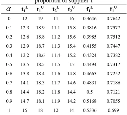
values. [image:6.595.45.287.156.654.2] [image:6.595.322.530.593.781.2]As we mentioned in Section III.A each supplier has different delivery time because of many reasons. For simplicity we name Mehvarsazan Company as supplier 1, and Farasanat as supplier 2. Our fuzzy delivery rate numbers are based on experts opinions, but the customer demand is obtained from historical data. The customer demand is approximated 100 axles per day. The economic quantity for every delivery is 10 numbers therefore we can consider numbers as standard batch, in other words
D
10
. We assume delivery rates for supplier 1 and 2 are trapezoid numbers. As experts proposed the supplier 1 can dispatch batches and the supplier 2 can dispatch batches per day. We want to find out how to split orders among tow suppliers in order to have minimized shortage cost. After performing numerical solutions for different
values, the shape of corresponding membership function can be approximated. The rough shape seems quite well and looks like a continuous function. The values of variables at different possibility levels and supplier 1 proportions are shown in Table.1, Table.2 and Fig. 3 illustrates the results of supplier 2 solution procedure.Table.1 of delivery rates and obtained proportion of supplier 1
f1U
f1L
t2U
t2L
t1U
t1L
Fig. 2. The membership function for fuzzy proportion of supplier 1
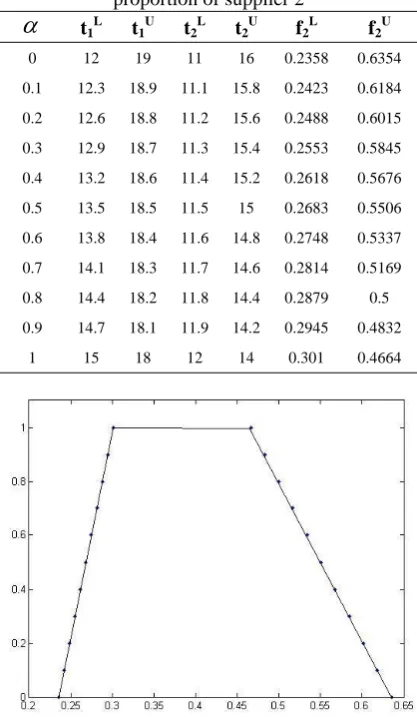
Table.2 of delivery rates and obtained proportion of supplier 2
f2U
f2L
t2U
t2L
t1U
t1L
0.6354 0.2358
16 11 19 12 0
0.6184 0.2423
15.8 11.1 18.9 12.3 0.1
0.6015 0.2488
15.6 11.2 18.8 12.6 0.2
0.5845 0.2553
15.4 11.3 18.7 12.9 0.3
0.5676 0.2618
15.2 11.4 18.6 13.2 0.4
0.5506 0.2683
15 11.5 18.5 13.5 0.5
0.5337 0.2748
14.8 11.6 18.4 13.8 0.6
0.5169 0.2814
14.6 11.7 18.3 14.1 0.7
0.5 0.2879 14.4
11.8 18.2 14.4 0.8
0.4832 0.2945
14.2 11.9 18.1 14.7 0.9
0.4664 0.301
14 12 18 15 1
Fig. 3 The membership function for fuzzy proportion of supplier 2
By replacing the above results in expression (12) we can obtain the fuzzy total cost, which can be defuzzied and get changed to crisp form. In this case after defuzzifying, total cost is obtained 1.01. Now we can compare this number with two different cases in order to ensure that the solution result is optimized. If we solve the problem in situations which just one of suppliers is considered for dispatching orders we will obtain two numbers. By considering supplier 1 proportion equal to 100% we obtain 2.50 as total cost. And similarly for supplier 2 we obtain 4.97. Therefore we
can confidently propose that the solution is optimized. V. CONCLUSION
In this paper we have studied on a new framework of order splitting problems in uncertain situations. We have analyzed the application of a fuzzy order splitting in a two level supply chain with purpose of minimizing the total cost. This study has shown that in the case of random demands from customers and fuzzy delivery delays from suppliers, it is generally useful to split the orders between several suppliers than to allocate all the replenishment orders to a single one and in such uncertain situations that we cannot approximate delivery rates based on historical data, fuzzy theory is a useful approach to be utilized. More specifically we solved the problem in a 2-suppliers case study (SAPCO) in MTO status to determine the percentages of orders to be allocated to each supplier; however the introduced technique has been proposed to solve the general N-suppliers case. We validated this technique by comparing the optimal solution in 2 supplier case with single sourcing case.
REFERENCES
[1] S.P. Chen,”Parametric nonlinear programming approach to fuzzy queues with bulk service”, European Journal of Operational Research 163, 2005, 434–444.
[2] J.J. Buckley,”Elementary queuing theory based on possibility theory,“ Fuzzy Sets and Systems 37, 1990, 43–52.
[3] J.J. Buckley, T. Feuring, Y. Hayashi,”Fuzzy queuing theory revisited”, International Journal of Uncertainty, Fuzziness, and Knowledge-Based Systems 9, 2001, 527–537.
[4] L.A. Zadeh,”Fuzzy sets as a basis for a theory of possibility”, Fuzzy Sets and Systems 1, 1978, 3–28.
[5] R.E. Stanford,”The set of limiting distributions for a Markov chain with fuzzy transition probabilities”, Fuzzy Sets and Systems 7, 1982, 71–78.
[6] R.J. Li, E.S. Lee,”Analysis of fuzzy queues”, Computers and Mathematics with Applications 17, 1989, 1143–1147.
[7] D.S. Negi, E.S. Lee,”Analysis and simulation of fuzzy queues”, Fuzzy Sets and Systems 46, 1992, 321–330.
[8] C. Kao, C.C. Li, S.P. Chen,” Parametric programming to the analysis of fuzzy queues”, Fuzzy Sets and Systems 107, 1999, 93–100. [9] N. Costantino, R. Pellegrino,”Choosing between single and multiple
sourcing based on supplier default risk: A real options approach”, Journal of Purchasing & Supply Management (2009).
[10] S. Axsater,”Inventory control”, Kluwer Academic Publishers, 2000. [11] H.J. Zimmermann,”Fuzzy Set Theory and its Application”, third ed.,
Kluwer Academic Publishers, 1996.
[12] Y. Arda, J.C. Hennet,”Inventory control in a multi-supplier system”, Int. J. Production Economics 104, 2006, 249–259.
[13] Y. Arda, J.C. Hennet,”optimizing the ordering policy in a supply chain”, LAAS Report 03492, 2003.
[image:7.595.63.274.265.629.2] [image:7.595.64.273.266.625.2]