Graph-based Neural Multi-Document Summarization
Michihiro Yasunaga1 Rui Zhang1 Kshitijh Meelu1 Ayush Pareek2 Krishnan Srinivasan1 Dragomir Radev1
1Department of Computer Science, Yale University 2The LNM Institute of Information Technology
{michihiro.yasunaga,r.zhang,kshitijh.meelu}@yale.edu {ayush.original}@gmail.com
{krishnan.srinivasan,dragomir.radev}@yale.edu
Abstract
We propose a neural multi-document sum-marization (MDS) system that incorpo-rates sentence relation graphs. We employ a Graph Convolutional Network (GCN) on the relation graphs, with sentence em-beddings obtained from Recurrent Neural Networks as input node features. Through multiple layer-wise propagation, the GCN generates high-level hidden sentence fea-tures for salience estimation. We then use a greedy heuristic to extract salient sen-tences while avoiding redundancy. In our experiments on DUC 2004, we consider three types of sentence relation graphs and demonstrate the advantage of combin-ing sentence relations in graphs with the representation power of deep neural net-works. Our model improves upon tradi-tional graph-based extractive approaches and the vanilla GRU sequence model with no graph, and it achieves competitive re-sults against other state-of-the-art multi-document summarization systems.
1 Introduction
Document summarization aims to produce fluent and coherent summaries covering salient informa-tion in the documents. Many previous summa-rization systems employ an extractive approach by identifying and concatenating the most salient text units (often whole sentences) in the document.
Traditional extractive summarizers produce the summary in two steps: sentence ranking and sentence selection. First, they utilize human-engineered features such as sentence position and length (Radev et al., 2004a), word frequency and importance (Nenkova et al.,2006;Hong and Nenkova, 2014), among others, to rank sentence
salience. Then, they select summary-worthy sen-tences using a range of algorithms, such as graph centrality (Erkan and Radev,2004), constraint op-timization via Integer Linear Programming (Mc-Donald, 2007; Gillick and Favre, 2009;Li et al., 2013), or Support Vector Regression (Li et al., 2007) algorithms. Optionally, sentence reordering (Lapata,2003;Barzilay et al.,2001) can follow to improve coherence of the summary.
Recently, thanks to their strong representation power, neural approaches have become popular in text summarization, especially in sentence com-pression (Rush et al.,2015) and single-document summarization (Cheng and Lapata,2016). Despite their popularity, neural networks still have issues when dealing with multi-document summarization (MDS). In previous neural multi-document sum-marizers (Cao et al.,2015,2017), all the sentences in the same document cluster are processed inde-pendently. Hence, the relationships between sen-tences and thus the relationships between differ-ent documdiffer-ents are ignored. However,Christensen et al.(2013) demonstrates the importance of con-sidering discourse relations among sentences in multi-document summarization.
This work proposes a multi-document summa-rization system that exploits the representational power of deep neural networks and the sentence relation information encoded in graph representa-tions of document clusters. Specifically, we apply Graph Convolutional Networks (Kipf and Welling, 2017) on sentence relation graphs. First, we dis-cuss three different techniques to produce sentence relation graphs, where nodes represent sentences in a cluster and edges capture the connections be-tween sentences. Given a relation graph, our sum-marization model apples a Graph Convolutional Network (GCN), which takes in sentence embed-dings from Recurrent Neural Networks as input node features. Through multiple layer-wise
agation, the GCN generates high-level hidden fea-tures for the sentences. We then obtain sentence salience estimations through a regression on top, and extract salient sentences in a greedy manner while avoiding redundancy.
We evaluate our model on the DUC 2004 multi-document summarization (MDS) task. Our model shows a clear advantage over traditional graph-based extractive summarizers, as well as a base-line GRU model that does not use any graph, and achieves competitive results with other state-of-the-art MDS systems. This work provides a new gateway to incorporating graph-based techniques into neural summarization.
2 Related Work 2.1 Graph-based MDS
Graph-based MDS models have traditionally em-ployed surface level (Erkan and Radev,2004; Mi-halcea and Tarau, 2005;Wan and Yang,2006) or deep level (Pardo et al., 2006; Antiqueira et al., 2009) approaches based on topological features and the number of nodes (Albert and Barab´asi, 2002). Efforts have been made to improve de-cision making of these systems by using dis-course relationships between sentences (Radev, 2000;Radev et al.,2001).Erkan and Radev(2004) introduce LexRank to compute sentence impor-tance based on the eigenvector centrality in the connectivity graph of inter-sentence cosine simi-larity. Mei et al.(2010) propose DivRank to bal-ance the prestige and diversity of the top ranked vertices in information networks and achieve im-proved results on MDS.Christensen et al.(2013) build multi-document graphs to identify pairwise ordering constraints over the sentences by ac-counting for discourse relationships between sen-tences (Mann and Thompson,1988). In our work, we build on the Approximate Discourse Graph (ADG) model (Christensen et al., 2013) and ac-count for macro level features in sentences to im-prove sentence salience prediction.
2.2 Summarization Using Neural Networks
Neural networks have recently been popular for text summarization (K˚ageb¨ack et al.,2014;Rush et al.,2015;Yin and Pei,2015;Cao et al.,2016; Wang and Ling, 2016;Cheng and Lapata, 2016; Nallapati et al.,2016,2017;See et al.,2017). For example, Rush et al. (2015) introduce a neural attention feed-forward network-based model for sentence compression. Wang and Ling (2016)
employ encoder-decoder RNNs to effectively pro-duce short abstractive summaries for opinions. Cao et al. (2016) develop a query-focused sum-marization system called AttSum which deals with saliency ranking and relevance ranking using query-attention-weighted CNNs.
Very recently, thanks to the large scale news article datasets (Hermann et al., 2015), Cheng and Lapata(2016) train an extractive summariza-tion system with attensummariza-tion-based encoder-decoder RNNs to sequentially label summary-worth sen-tences in single documents. See et al. (2017), adopting an abstractive approach, augment the standard attention-based encoder-decoder RNNs with the ability to copy words from the source text via pointing and to keep track of what has been summarized. These models (Cheng and Lapata, 2016;See et al.,2017) achieve state-of-the-art per-formance on the DUC 2002 single-document sum-marization task. However, scaling up these RNN sequence-to-sequence approaches to the multi-document summarization task has not been suc-cessful, 1) due to the lack of large multi-document summarization datasets needed to train the compu-tationally expensive sequence-to-sequence model, and 2) because of the inadequacy of RNNs to cap-ture the complex discourse relations across multi-ple documents. Our multi-document summariza-tion model resolves these issues 1) by breaking down the summarization task into salience estima-tion and sentence selecestima-tion that do not require an expensive decoder architecture, and 2) by utilizing sentence relation graphs.
3 Method
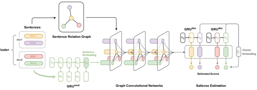
Given a document cluster, our method extracts sentences as a summary in two steps: sentence salience estimation and sentence selection. Figure 1illustrates our architecture for sentence salience estimation. Given a document cluster, we first build a sentence relation graph, where interact-ing sentence nodes are connected by edges. For each sentence, we apply an RNN with Gated Re-current Units (GRUsent) (Cho et al.,2014;Chung
pdfcrowd.com PRO version Are you a developer? Try out the HTML to PDF API
w1 h1 h2
w2
h3
w3
h4
.
Sentences
GRUsent
Sentence Relation Graph
h0
Graph Convolutional Networks Salience Estimation h1 h2 h1 h2
h0
C Sentence
Embedding
Cluster Embedding
Estimated Scores
GRUdoc
Cluster
h0
GRUdoc
doc1
d1s1
d1s2
doc2 d2s1
[image:3.595.76.524.63.220.2]d2s2
Figure 1: Illustration of our architecture for sentence salience estimation. In this example, there are two documents in the cluster and each document has two sentences. Sentences are processed by theGRUsent
to get input sentence embeddings. The GCN takes the input sentence embeddings and the sentence relation graph, and outputs high-level hidden features for individual sentences. GRUdoc produces the
cluster embedding from the output sentence embeddings. The salience is estimated from the output sentence embeddings and the cluster embedding. wi: the word embedding fori-th word. hi: the hidden
state ofGRUati-th step.
by sequentially connecting the final sentence em-beddings. We estimate the salience of each sen-tence from the final sensen-tence embeddings and the cluster embedding. Finally, based on the estimated salience scores, we select sentences in a greedy way until reaching the length limit.
3.1 Graph Representation of Clusters
To best evaluate the architecture, we consider three graph representation methods to model sen-tence relationships within clusters. First, as prior methods in representing document clusters often adhere to the standard of cosine similarity (Erkan and Radev, 2004), our initial baseline approach naturally used this representation. Specifically, we add an edge between two sentences if the tf-idf co-sine similarity measure between them, using the bag-of-words model, is above a threshold of 0.2.
Secondly, the G-Flow system (Christensen et al., 2013) utilizes discourse relationships be-tween sentences to create its graph representa-tions, known as Approximate Discourse Graph (ADG). The ADG constructs edges between sen-tences by counting discourse relation indicators such as deverbal noun references, event and entity continuations, discourse markers, and co-referent mentions. These features allow characterization of sentence relationships, rather than simply their similarity.
While G-Flow’s ADG provides many improve-ments from baseline graph representations, it suf-fers several disadvantages that diminish its ability
Personalization Features • Position in Document
• From1st3Sentences?
• No. of Proper Nouns • >20 Tokens in Sentence? • Sentence Length
• No. of Co-referent Verb Mentions
• No. of Co-referent Common Noun Mentions • No. of Co-referent Proper Noun Mentions
Table 1: List of features that were input to the re-gression function in obtaining sentence personal-ization scores.
A baseline sentence personalization scores(v), which can be viewed as weighting of sentences, is calculated for every sentence v to account for surface features in each sentence. These features, listed in Table 1, are used as input for linear re-gression, as perChristensen et al.(2013). The re-gression is applied to each sentence to obtain the personalization score,s(v). Each edge weight in the original ADG is then transformed by this sen-tence personalization score and normalized over the total outgoing scores. That is, for directed edge
(u, v)∈E, the weight is
wP DG(u, v) = P wADG(u, v)s(v)
u0∈V wADG(u0, v)s(u0) (1) The inclusion of the sentence personalization scores allows the PDG to account for macro-level features in each sentence, augmenting information for salience estimation. To provide more clarity, we include a figure of the PDG in later sections.
Although it may be possible to incorporate the sentence personalization features later into the salience estimation network, we chose to encode them in the PDG to improve the edge weight dis-tribution of sentence relation graphs and to make our salience estimation architecture methodically consistent. Additionally, in order to maintain con-sistency between graph representations, follow-ing two modifications are made to the discourse graphs. First, the directed edges of both the ADG and PDG are made undirected by averaging the edges weights in both directions. Second, edge weights are rescaled to a maximum edge weight of 1 prior to being fed to the GCN.
3.2 Graph Convolutional Networks
We apply Graph Convolutional Networks (GCN) fromKipf and Welling (2017) on top of the sen-tence relation graph. In this subsection, we ex-plain in detail the formulation of GCN, and how GCN produces the final sentence embeddings.
The goal of GCN is to learn a functionf(X, A)
that takes as input:
• A ∈RN×N, the adjacency matrix of graphG,
whereN is the number of nodes inG.
• X ∈ RN×D, the input node feature matrix,
whereDis the dimension of input node feature vectors.
and outputs high-level hidden features for each node, Z ∈ RN×F, that encapsulate the graph
structure. F is the dimension of output feature
vectors. The function f(X, A) takes a form of layer-wise propagation based on neural networks. We compute the activation matrix in the(l+ 1)th
layer asH(l+1), starting fromH0 = X. The
out-put ofL-layer GCN isZ =f(X, A) =H(L).
To introduce the formulation, consider a simple form of layer-wise propagation:
H(l+1)=σAH(l)W(l) (2)
whereσis an activation function such asReLU(·) = max(0,·).W(l)is the parameter to learn in the
lth layer. Eq 2 has two limitations. First,
mul-tiplying byA means that for each node, we sum up the feature vectors of all neighboring nodes but not the node itself. We fix this by adding self-loops in the graph. Second, sinceAis not normalized, multiplying byAwill change the scale of feature vectors. To overcome this, we apply a symmet-ric normalization by usingD−1
2AD−12 whereD
is the node degree matrix. These two renormaliza-tion tricks result in the following propagarenormaliza-tion rule:
H(l+1)=σD˜−1
2A˜D˜−12H(l)W(l)
(3)
where A˜ = A +IN is the adjacency matrix of
the graphGwith added self-loops (IN is the
iden-tity matrix). D˜ is the degree matrix with D˜ii =
P
jA˜ij. Kipf and Welling(2017) also provide a
theoretical justification of Eq3as a first-order ap-proximation of spectral graph convolution (Ham-mond et al.,2011;Defferrard et al.,2016).
As an example, if we have a two-layer GCN, we first calculate Aˆ = ˜D−1
2A˜D˜−12 in a
pre-processing step, and then produce
Z =f(X, A) =σA σˆ AXWˆ (0)W(1)
3.3 Sentence Embeddings
As the input node featuresXof GCN, we use sen-tence embeddings calculated byGRUsent.
Given a document cluster C withN sentences
(s1, s2, ..., sN) in total, for each sentencesi ofL
words(w1, w2, ..., wL), GRUsent recurrently
up-dates hidden states at each time stept:
hsentt = GRUsent(hsentt−1,wt) (4)
wherewt is the word embedding forwt,hsentt is
the hidden state ofGRUsent. h
0 is initialized as a
zero vector, and the input sentence embeddingxi
is the last hidden state:
All sentence embeddings from the given document cluster are grouped as the node feature matrixX:
X=
xT
1
xT
2
...
xT N
(6)
Xis fed into GCN subsequently to obtain the final sentence embeddingssithat incorporate the graph
representation of sentence relationships:
Z =f(X, A) =
sT
1
sT
2
...
sT N
(7)
3.4 Cluster Embedding
Additionally, in order to have a global view of the entire document cluster, we apply a second-level RNN, GRUdoc, to encode the entire docu-ment cluster. Given a docudocu-ment clusterCwithM documents(d1, d2, ..., dM), for documentdi with
|di|sentences, GRUdoc first builds the document
embeddingdion top of sentence embeddings: hdoc
t = GRUdoc(hdoct−1,st) (8) di=hdoc|di| (9)
where st is the sentence embedding in the
docu-mentdi. In Eq 9, we extract the last hidden state
as the document embedding fordi. In Eq10, we
average over document embeddings to produce the cluster embeddingC:
C= M1 M
X
i=1
di (10)
All the GRUs we used are forward. We also exper-imented with backward GRUs and bi-directional GRUs, but neither of them meaningfully improved upon forward GRUs.
3.5 Salience Estimation
For the sentencesi in the clusterC, we calculate
the salience ofsias the following, similarly to the
attention mechanism in neural machine translation (Bahdanau et al.,2015):
f(si) =vT tanh(W1C+W2si) (11) salience(si) = P f(si)
sj∈Cf(sj) (12)
where v,W1,W2 are learnable parameters. In
Eq 11, we first calculate the scoref(si) by
con-sidering the sentence embedding itself,si, and the
cluster embeddingCfor the global context of the multi-document. The score is then normalized as
salience(si)via softmax in Eq12. 3.6 Training
The model parameters include the parameters in GRUsent and GRUdoc, the weights in GCN layers, and the parameters for salience estima-tion (v,W1,W2). Parameters in GRUsent and
GRUdocare not shared. The model is trained end-to-end to minimize the following cross-entropy loss between the salience prediction and the nor-malized ROUGE score of each sentence:
L=−X
C
X
si∈C
R(si) log(salience(si)) (13)
R(si)is calculated byR(si) = softmax(α r(si)),
where r(si) is the average of ROUGE-1 and
ROUGE-2 Recall scores of sentence si by
mea-suring with the ground-truth human-written sum-maries.αis a constant rescaling factor to make the distribution sharper. The value ofαis determined from the validation data set. αr(si) is then
nor-malized across the cluster via softmax, similarly to Eq12.
3.7 Sentence Selection
Given the salience score estimation, we apply a simple greedy procedure to select sentences. Sen-tences with higher salience scores have higher pri-orities. First, we sort sentences in descending or-der of the salience scores. Then, we select one sentence from the top of the list and append to the summary if the sentence is of reasonable length (8-55 words, as in (Erkan and Radev,2004)) and is not redundant. The sentence is redundant if the tf-idf cosine similarity between the sentence and the current summary is above 0.5 (Hong and Nenkova, 2014). We select sentences this way until we reach the length limit.
4 Experiments
DUC’01 DUC’02 DUC’03 DUC’04
# of Clusters 30 59 30 50
# of Documents 309 567 298 500
# of Sentences 24498 16090 7721 13270
Vocabulary Size 28188 22174 13248 18036
[image:6.595.308.522.63.266.2]Summary Length words100 words100 words100 Bytes665
Table 2: Statistics for DUC Multi-Document Sum-marization Data Sets.
we further study the effect of graph and different graph representations on the summarization per-formance and investigate the correlation of graph structure and sentence salience estimation.
4.1 Data Set and Evaluation
We use the benchmark data sets from the Docu-ment Understanding Conferences (DUC) contain-ing clusters of English news articles and human reference summaries. Table2shows the statistics of the data sets. We use DUC 2001, 2002, 2003 and 2004 containing 30, 59, 30 and 50 clusters of nearly 10 documents each respectively. Our model is trained on DUC 2001 and 2002, validated on 2003, and tested on 2004. For evaluation, we use the ROUGE-1,2 metric, with stemming and stop words not removed as suggested by Owczarzak et al.(2012).
4.2 Experimental Setup
We conduct four experiments on our model: three using each of the three types of graphs discussed earlier, and one without using any graph. In the experiments with graphs, for each document clus-ter, we tokenize all the documents into sentences and generate a graph representation of their re-lations by the three methods: Cosine Similar-ity Graph, Approximate Discourse Graph (ADG) from G-Flow, and our Personalized Discourse Graph (PDG). Note that for the Cosine Similar-ity Graph, we compute the tf-idf cosine similarSimilar-ity for every pair of sentences using the bag-of-word model and add an edge for similarity above 0.2. The weight of the edge is the value of similarity. We apply GCNs with the graphs in the final step of sentence encoding. For the experiment without any graph, we omit the GCN part and simply use the GRU sentence and cluster encoders.
We use 300-dimensional pre-trained word2vec embeddings (Mikolov et al., 2013) as input to
GRUsentin Eq4. The word embeddings are fine-tuned during training. We use three GCN hidden
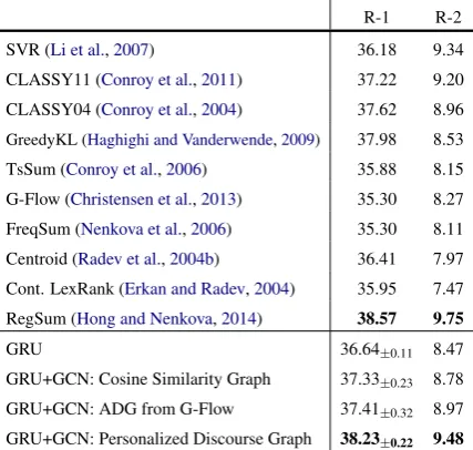
R-1 R-2
SVR (Li et al.,2007) 36.18 9.34
CLASSY11 (Conroy et al.,2011) 37.22 9.20 CLASSY04 (Conroy et al.,2004) 37.62 8.96 GreedyKL (Haghighi and Vanderwende,2009) 37.98 8.53 TsSum (Conroy et al.,2006) 35.88 8.15 G-Flow (Christensen et al.,2013) 35.30 8.27 FreqSum (Nenkova et al.,2006) 35.30 8.11 Centroid (Radev et al.,2004b) 36.41 7.97 Cont. LexRank (Erkan and Radev,2004) 35.95 7.47 RegSum (Hong and Nenkova,2014) 38.57 9.75
GRU 36.64±0.11 8.47
GRU+GCN: Cosine Similarity Graph 37.33±0.23 8.78
GRU+GCN: ADG from G-Flow 37.41±0.32 8.97
GRU+GCN: Personalized Discourse Graph 38.23±0.22 9.48
Table 3: ROUGE Recalls on DUC 2004. We show mean (and standard deviation for R-1) over 10 re-peated trials for each of our experiments.
layers (L = 3). The hidden states in GRUsent,
GCN hidden layers, and GRUdoc are all
300-dimensional vectors (D=F = 300).
The rescaling factor α in the objective func-tion (Eq 13) is chosen as 40 from {10, 20, 30, 40, 50, 100}based on the validation performance. The objective function is optimized using Adam (Kingma and Ba, 2015) stochastic gradient de-scent with a learning rate of 0.001 and a batch size of 1. We use gradient clipping with a maximum gradient norm of 1.0. The model is validated ev-ery 10 iterations, and the training is stopped early if the validation performance does not improve for 10 consecutive steps. We trained using a single Tesla K80 GPU. For all the experiments, the train-ing took approximately 30 minutes until a stop.
4.3 Results
Table3summarizes our results. First we take our simple GRU model as the baseline of the RNN-based regression approach. As seen from the table, the addition of Cosine Similarity Graph on top of the GRU clearly boosts the performance. Further-more, the addition of ADG from G-Flow gives a slighly better performance. Our Personalized Dis-course Graph (PDG) enhances the R-1 score by more than 1.50. The improvement indicates that the combination of graphs and GCNs processes sentence relations across documents better than the vanilla RNN sequence models.
[image:6.595.75.288.63.158.2]state-of-the-PDG ADG SimilarityCosine GraphNo Num of Iterations 200 280 310 250 Train Cost 4.286 5.460 5.458 5.310 Validation Cost 4.559 5.077 5.099 5.214
Table 4: Training statistics for the four experi-ments. The first row shows the number of itera-tions the model took to reach the best validation result before an early stop. The train cost and val-idation cost at that time step are shown in the sec-ond row and third row, respectively. All the values are the average over 10 repeated trials.
art systems related to our regression method. We compute ROUGE scores from the actual output summary of each system. We run the G-Flow code released by Christensen et al. (2013) to get the output summary of the G-Flow system. The output summary of other systems are compiled in Hong et al.(2014). To ensure fair comparison, we use ROUGE-1.5.5 with the same parameters as in Hong et al.(2014) across all methods: -n 2 -m -l 100 -x -c 95 -r 1000 -f A -p 0.5 -t 0.
From Table 3, we observe that our GCN sys-tem significantly outperforms the commonly used baselines and traditional graph approaches such as Centroid, LexRank, and G-Flow. This indi-cates the advantage of the representation power of neural networks used in our model. Our tem also exceeds CLASSY04, the best peer sys-tem in DUC 2004, and Support Vector Regres-sion (SVR), a widely used regresRegres-sion-based sum-marizer. We remain at a comparable level to Reg-Sum, the state-of-the-art multi-document summa-rizer using regression. The major difference is that RegSum performs regression on word level and estimates the salience of each word through a rich set of word features, such as frequency, gram-mar, context, and hand-crafted dictionaries. Reg-Sum then computes sentence salience based on the word scores. On the other hand, our model simply works on sentence level, spotlighting sentence re-lations encoded as a graph. Incorporating more word-level features into our discourse graphs may be an interesting future direction to explore.
4.4 Discussion
As shown in Table 3, our graph-based models outperform the vanilla GRU model, which has no graph. Additionally, for the three graphs we consider, PDG improves R-1 score by 0.82 over ADG, and ADG outperforms the Cosine
Similar-0 50 100 150 200 250 300 350 400
4 4.5 5 5.5 6 6.5 7
Number of Iterations
V
alidation
Cost
No Graph Similarity Graph ADG
[image:7.595.311.520.63.203.2]PDG
Figure 1: Learning curves of the four experiments based on the validation costs. Note that the vertical axis is only displaying the interval 4.0 - 7.0.
1
Introduction
1
Figure 2: Visualization of the learning curves for the four experiments. The vertical axis displays the validation costs in the interval 4.0 - 7.0.
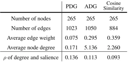
PDG ADG SimilarityCosine Number of nodes 265 265 265 Number of edges 1023 1050 884 Average edge weight 0.075 0.295 0.359 Average node degree 0.171 5.136 2.260
ρof degree and salience 0.136 0.113 0.093
Table 5: Characteristics of the three graph repre-sentations, averaged over the clusters (i.e. graphs) in DUC 2004. Note that max edge weight in all three representations is 1.0 due to rescaling for consistency. The degree of each node is calculated as the sum of edge weights.
ity Graph by 0.08 on the R-1 score. While the Co-sine Similarity Graph encodes general word-level connections between sentences, discourse graphs, especially our personalized version, specialize in representing the narrative and logical relations be-tween sentences. Therefore, we hypothesize that the PDG provides a more informative guide to es-timating the importance of each sentence. In an at-tempt to better understand the results and validate the effect of sentence relation graphs (especially of the PDG), we have conducted the analysis that follows.
[image:7.595.309.523.263.366.2]0.00 0.05 0.10 0.15 0.20 0.25 0.30 Salience scores
Correlation Coefficient: 0.45 0.0
0.5 1.0 1.5 2.0
Node Degrees
PDG
0.00 0.05 0.10 0.15 0.20 0.25 0.30 Salience scores
Correlation Coefficient: 0.37 0
5 10 15 20 25 30 35 40 45
Node Degrees
ADG
0.00 0.05 0.10 0.15 0.20 0.25 0.30 Salience scores
Correlation Coefficient: 0.13 0
1 2 3 4 5 6
Node Degrees
[image:8.595.73.520.66.173.2]Similarity Graph
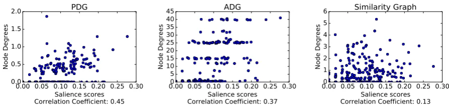
Figure 3: Visualization of the relationship between salience score and node degree for the three graph representation methods. Cluster d30011t from DUC 2004 is chosen as an example.
than the models with graphs. For the three graph methods, ADG converges faster and has better validation performance than the Cosine Similar-ity Graph. PDG converges even faster than “No Graph” and achieves the lowest training cost and validation cost amongst all methods. This shows that the PDG has particularly strong representation power and generalizability.
Graph Statistics. We also analyze the charac-teristics of the three graph representation methods on DUC 2004 document clusters. Table5 summa-rizes the following basic statistics: the number of nodes (i.e. sentences), the number of edges, av-erage edge weight, and avav-erage node degree per graph. We include the correlation between node degree and salience, as well.
As seen from the table, PDG and ADG have ap-proximately the same number of edges. This is expected since the PDG is built by transforming the edge weights in ADG. The Cosine Similarity Graph has slightly fewer edges, simply due to the implemented threshold.
Moreover, note that the ADG has significantly higher average edge weight and node degree as compared to the PDG. These values reflect the discrete nature of the ADG’s edge assignment — further evidence of this can be seen in Figure 3. Because the ADG’s raw edge weight assignment is done by increments of 0.5, the average node degree tends to be significantly large. This mo-tivated the construction of our PDG, which cor-rects for this by coercing the average edge weight and node degree to be more diverse and, conse-quently, smaller (after rescaling). The process of including sentence personalization scores in edge weight assignments of the PDG leads to a select number of edges gaining markedly large distinc-tion. This aids the GCN in identifying the most important edge connections along with the
affili-ated sentences.
Node Degree and Salience. In Table5, we also calculate the correlation coefficient ρ, per graph, between the degree of each sentence node and its salience score. We observe that all the graph rep-resentations show positive correlation between the node degree and the salience score. Moreover, the order of correlation strength is PDG>ADG> Co-sine Similarity Graph. Though node degree is a simple measure of these graphs, this observation supports our hypothesis on the efficacy of sentence relation graphs, particularly of PDGs, to provide a guide to salience estimation.1
As a case study to illustrate our observation, we chose one cluster (d30011t) from DUC 2004. Fig-ure 3 shows the scatter plots of the node degree and salience score of each sentence.
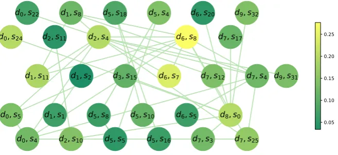
Visualization of the PDG. Finally, to demon-strate the functionality of the PDG and comple-ment our discussion from Section 3.1, we visual-ize the PDG on cluster d30011t with the salience score on each node in Figure4(also see Figure5 for the actual sentences).
From the visualization, it can be observed that the nodes representing salient sentences (such as (d6, s8), (d6, s7), and (d2, s4)) tend to have higher
degrees in the PDG. We can also observe that the PDG represents edges which connect nodes of sentences from different documents, in contrast with the traditional sequence model.
From Figure 5, we note that the most salient sentence (d6, s8) actually describes much of the
reference summary. As an example of discourse relation, (d6, s7) and (d2, s4), the two nodes
con-nected to (d6, s8), provide the background for
1 However, we shall add that simply selecting sentences
Figure 4: Visualization of the PDG on cluster d30011t. Each node is a sentence, with label (DocumentID, SentenceID). The node color represents the salience score (see the color bar). For simplicity, we only display edges of weight above 0.03. Best viewed in color.
Reference Summary (truncated): Malaysian
Prime Minister Mahathir Mohamad ruled adroitly for 17 years until September 1998 when he
suddenly reversed his economic policy and fired
his popular deputy and heir apparent, Anwar
Ibrahim. Anwar organized a political opposition,
leading Mahathir to arrest him. (...) Anwar
remained in custody as lawyers appealed. (...)
Sent-label (6,8): Anwar was ... after two weeks of nationwide rallies at which he called for
government reform and Mahathir's resignation,
he was arrested ....
Sent-label (6,7): The two had differed over
economic policy and Anwar has said Mahathir feared he was a threat to his 17-year rule.
Sent-label (2,4): Mahathir and Anwar had
differed over economic policy and Anwar says
Mahathir feared him as an alternative leader.
Sent-label (0,22): Before his arrest, Anwar designated his wife, Azizah Ismail, as the leader of his new ``reform'' movement.
Figure 5: Reference summary and illustrative sen-tences from cluster d30011t.
(d6, s8), even though they do not share many
words in common with it. On the other hand, (d0, s22), which is only connected with (d2, s4), is
not salient as it does not provide a central message for the summary.
5 Conclusion
In this paper, we presented a novel multi-document summarization system that exploits the represen-tational power of neural networks and graph rep-resentations of sentence relationships. On top of a simple GRU model as an RNN-based regression
baseline, we build a Graph Convolutional Network (GCN) architecture applied on a Personalized Dis-course Graph. Our model, unlike traditional RNN models, can capture sentence relations across doc-uments and demonstrates improved salience pre-diction and summarization, achieving competitive performance with current state-of-the-art systems. Furthermore, through multiple analyses, we have validated the efficacy of sentence relation graphs, particularly of PDG, to help to learn the salience of sentences. This work shows the promise of the GCN models and of discourse graphs applied to processing multi-document inputs.
Acknowledgements
We would like to thank the members of the Sap-phire Project (University of Michigan and IBM), as well as all the anonymous reviewers for their helpful suggestions on this work. This material is based in part upon work supported by IBM under contract 4915012629. Any opinions, find-ings, conclusions, or recommendations expressed herein are those of the authors and do not neces-sarily reflect the views of IBM.
References
R´eka Albert and Albert-L´aszl´o Barab´asi. 2002. Statis-tical mechanics of complex networks. Reviews of
modern physics74(1):47.
Lucas Antiqueira, Osvaldo N Oliveira, Luciano da Fon-toura Costa, and Maria das Grac¸as Volpe Nunes. 2009. A complex network approach to text summa-rization. Information Sciences179(5):584–599.
Ben-gio. 2015. Neural machine translation by jointly learning to align and translate. InICLR.
Regina Barzilay, Noemie Elhadad, and Kathleen R McKeown. 2001. Sentence ordering in multidocu-ment summarization. InProceedings of the first in-ternational conference on Human language
technol-ogy research.
Ziqiang Cao, Wenjie Li, Sujian Li, and Furu Wei. 2017. Improving multi-document summarization via text classification. InAAAI.
Ziqiang Cao, Wenjie Li, Sujian Li, Furu Wei, and Yan-ran Li. 2016. Attsum: Joint learning of focusing and summarization with neural attention. InCOLING. Ziqiang Cao, Furu Wei, Li Dong, Sujian Li, and Ming
Zhou. 2015. Ranking with recursive neural net-works and its application to multi-document sum-marization. InAAAI.
Jianpeng Cheng and Mirella Lapata. 2016. Neural summarization by extracting sentences and words. InACL.
Kyunghyun Cho, Bart van Merrienboer, Caglar Gul-cehre, Dzmitry Bahdanau, Fethi Bougares, Holger Schwenk, and Yoshua Bengio. 2014. Learning phrase representations using rnn encoder–decoder for statistical machine translation. InEMNLP. Janara Christensen, Mausam, Stephen Soderland, and
Oren Etzioni. 2013. Towards coherent multi-document summarization. InNAACL.
Junyoung Chung, Caglar Gulcehre, KyungHyun Cho, and Yoshua Bengio. 2014. Empirical evaluation of gated recurrent neural networks on sequence
model-ing. NIPS 2014 Deep Learning and Representation
Learning Workshop.
John M Conroy, Judith D Schlesinger, Jade Gold-stein, and Dianne P Oleary. 2004. Left-brain/right-brain multi-document summarization. In Proceed-ings of the Document Understanding Conference
(DUC 2004).
John M Conroy, Judith D Schlesinger, Jeff Kubina, Pe-ter A Rankel, and Dianne P O’Leary. 2011. Classy 2011 at tac: Guided and multi-lingual summaries and evaluation metrics. TAC11:1–8.
John M Conroy, Judith D Schlesinger, and Dianne P O’Leary. 2006. Topic-focused multi-document summarization using an approximate oracle score.
InCOLING/ACL.
Micha¨el Defferrard, Xavier Bresson, and Pierre Van-dergheynst. 2016. Convolutional neural networks on graphs with fast localized spectral filtering. InNIPS. G¨unes Erkan and Dragomir R Radev. 2004. Lexrank: Graph-based lexical centrality as salience in text summarization. Journal of Artificial Intelligence
Research22:457–479.
Dan Gillick and Benoit Favre. 2009. A scalable global model for summarization. In Proceedings of the Workshop on Integer Linear Programming for
Nat-ural Langauge Processing. Association for
Compu-tational Linguistics, pages 10–18.
Aria Haghighi and Lucy Vanderwende. 2009. Explor-ing content models for multi-document summariza-tion. InNAACL.
David K Hammond, Pierre Vandergheynst, and R´emi Gribonval. 2011. Wavelets on graphs via spec-tral graph theory. Applied and Computational
Har-monic Analysis30(2):129–150.
Karl Moritz Hermann, Tomas Kocisky, Edward Grefenstette, Lasse Espeholt, Will Kay, Mustafa Su-leyman, and Phil Blunsom. 2015. Teaching ma-chines to read and comprehend. InNIPS.
Kai Hong, John M Conroy, Benoit Favre, Alex Kulesza, Hui Lin, and Ani Nenkova. 2014. A repos-itory of state of the art and competitive baseline sum-maries for generic news summarization. InLREC. Kai Hong and Ani Nenkova. 2014. Improving the
estimation of word importance for news multi-document summarization. InEACL.
Mikael K˚ageb¨ack, Olof Mogren, Nina Tahmasebi, and Devdatt Dubhashi. 2014. Extractive summariza-tion using continuous vector space models. In Pro-ceedings of the 2nd Workshop on Continuous Vector Space Models and their Compositionality (CVSC)@ EACL. Citeseer, pages 31–39.
Diederik Kingma and Jimmy Ba. 2015. Adam: A method for stochastic optimization. InICLR. Thomas N Kipf and Max Welling. 2017.
Semi-supervised classification with graph convolutional networks. InICLR.
Mirella Lapata. 2003. Probabilistic text structuring: Experiments with sentence ordering. InACL. Chen Li, Xian Qian, and Yang Liu. 2013. Using
super-vised bigram-based ilp for extractive summarization. InACL.
Sujian Li, You Ouyang, Wei Wang, and Bin Sun. 2007. Multi-document summarization using support vec-tor regression. InProceedings of DUC. Citeseer. William C Mann and Sandra A Thompson. 1988.
Rhetorical structure theory: Toward a functional the-ory of text organization. Text-Interdisciplinary
Jour-nal for the Study of Discourse8(3):243–281.
Ryan McDonald. 2007. A study of global inference al-gorithms in multi-document summarization. In
Eu-ropean Conference on Information Retrieval.
Rada Mihalcea and Paul Tarau. 2005. A language inde-pendent algorithm for single and multiple document summarization. InIJCNLP.
Tomas Mikolov, Ilya Sutskever, Kai Chen, Greg S Cor-rado, and Jeff Dean. 2013. Distributed representa-tions of words and phrases and their compositional-ity. InNIPS.
Ramesh Nallapati, Feifei Zhai, and Bowen Zhou. 2017. Summarunner: A recurrent neural network based se-quence model for extractive summarization of docu-ments. AAAI.
Ramesh Nallapati, Bowen Zhou, Caglar Gulcehre, Bing Xiang, et al. 2016. Abstractive text summa-rization using sequence-to-sequence rnns and be-yond. InCoNLL.
Ani Nenkova, Lucy Vanderwende, and Kathleen McK-eown. 2006. A compositional context sensitive multi-document summarizer: exploring the factors that influence summarization. InSIGIR.
Karolina Owczarzak, John M Conroy, Hoa Trang Dang, and Ani Nenkova. 2012. An assessment of the accuracy of automatic evaluation in summariza-tion. In Proceedings of Workshop on Evaluation Metrics and System Comparison for Automatic
Sum-marization. Association for Computational
Linguis-tics, pages 1–9.
Thiago Pardo, Lucas Antiqueira, Maria Nunes, Os-valdo Oliveira, and Luciano da Fontoura Costa. 2006. Modeling and evaluating summaries using complex networks. Computational Processing of
the Portuguese Languagepages 1–10.
Dragomir R Radev. 2000. A common theory of infor-mation fusion from multiple text sources step one: cross-document structure. In Proceedings of the 1st SIGdial workshop on Discourse and
dialogue-Volume 10. Association for Computational
Linguis-tics, pages 74–83.
Dragomir R Radev, Timothy Allison, Sasha Blair-Goldensohn, John Blitzer, Arda Celebi, Stanko Dimitrov, Elliott Drabek, Ali Hakim, Wai Lam, Danyu Liu, et al. 2004a. Mead-a platform for multidocument multilingual text summarization. In
LREC.
Dragomir R Radev, Sasha Blair-Goldensohn, Zhu Zhang, and Revathi Sundara Raghavan. 2001. Newsinessence: A system for domain-independent, real-time news clustering and multi-document sum-marization. In Proceedings of the first interna-tional conference on Human language technology
research. Association for Computational
Linguis-tics, pages 1–4.
Dragomir R Radev, Hongyan Jing, Małgorzata Sty´s, and Daniel Tam. 2004b. Centroid-based summa-rization of multiple documents. Information
Pro-cessing & Management40(6):919–938.
Alexander M Rush, Sumit Chopra, and Jason Weston. 2015. A neural attention model for abstractive sen-tence summarization. InEMNLP.
Abigail See, Peter J. Liu, and Christopher D. Manning. 2017. Get to the point: Summarization with pointer-generator networks. InACL.
Xiaojun Wan and Jianwu Yang. 2006. Improved affin-ity graph based multi-document summarization. In
NAACL.
Lu Wang and Wang Ling. 2016. Neural network-based abstract generation for opinions and arguments. In
NAACL.