Numerical Approximations of Average Run Length for AR(1) on Exponential CUSUM



Abstract— We study the Cumulative Sum (CUSUM) procedure when observations are from a first order autoregressive model with exponential white noise. The objective of this paper is to present a numerical integration method for evaluating ARL₀ and ARL₁, where ARL₀ is the average run length when the process is in control and ARL1is the average run length when the process is out of control. The integrals in the Integral Equation (IE) method for the CUSUM procedure are approximated by using the Gauss-Legendre rule for numerical integration. The results obtained from the numerical integration method are compared with results obtained from explicit formulae. We have shown that the results obtained from the two methods are in excellent agreement.

Index Terms— Cumulative Sum, First order autoregressive, Average Run Length, Exponential distribution, Integral Equation.

I. INTRODUCTION

Statistical Process Control (SPC) is widely used to detect and monitor process changes in many areas such as industrial manufacturing [18], finance and economics [9], computer science and telecommunications [19], [23], epidemiology and surveillance [10], [25], [32] and in other areas of applications. Various SPC charts have been developed and extensively studied, for example, Shewhart [24], Exponentially Weighted Moving Average (EWMA) procedure [22] and Cumulative Sum (CUSUM) chart [21], [14]. A traditional assumption for evaluating the characteristics of SPC charts is that variables are random, independent and identically distributed. However, in practice, observations are not always identically and independently distributed (i.i.d.), for example, in continuous

This work was supported in part by the U.S. Department of Commerce under Grant BS123456 (sponsor and financial support acknowledgment goes here).

J. Busaba is with the King Mongkut’s University of Technology North Bangkok, Faculty of Applied Science, Department of Applied Statistics, Bangkok, Thailand, e-mail: [email protected]).

S. Sukparungsee is with the King Mongkut’s University of Technology North Bangkok, Faculty of Applied Science, Department of Applied Statistics, Bangkok, Thailand, e-mail: [email protected])

Y. Areepong is with the King Mongkut’s University of Technology North Bangkok, Faculty of Applied Science, Department of Applied

manufacturing processes where most observations are sequentially autocorrelated. Many SPC procedures have been developed to detect changes of mean and dispersion in autocorrelated manufacturing processes (see [1], [2], [4], [13], [16], [20], [23], [29], [30], [31]). However, these authors have used simulations and not analytical methods for determining the ARL. Simulation is commonly used to analyse the characteristics of methods which measure the number of observations that are required in order to decide if a stochastic process has changed from an in-control to an out-of-control state. In the past decade, many approaches have been developed for comparing the performance of SPC charts, for example, the Monte Carlo (MC), IE [7], Markov Chain Approach (MCA) [17] and Martingale approach [26, 27].

In this article, we study the ARLs of the CUSUM procedure when observations are from a first order autoregressive model with exponential white noise. We derive integral equations for the ARLs and then solve the equations numerically using the Gauss-Legendre numerical integration rule. We then compare the results obtained from the numerical integration method with the results from explicit formulae derived in [6].

The outline of the paper is as follows. In sections 2 and 3, we describe the characteristics of the SPC procedures and the properties of the CUSUM chart. In sections 4 and 5, we describe the numerical integral equation approach and show the numerical results. Section 6 contains a discussion and conclusions.

II. THE CHARACTERISTICS OF SPC PROCEDURES In this paper, we discuss the characteristics of SPC procedures based on the assumption that  1, 2,...,n are

sequentially observed identically distributed independent random variables with an exponential distribution function

Numerical Approximations of Average Run

Length for AR(1) on Exponential CUSUM

)

,

(

x



F

. We assume that the parameter



has the value 0



in the in-control state, the value







0 in an out-of-control state, and that the change occurs at a change-point time  . We assume that the parameters of the in-control and out-of-control states are known.

A typical method of detecting change points in SPC charts is to define some statistic

X

_n and a control boundary limit

h

of

X

_n such that an alarm signal is given when

X

_n exceeds

h

.

Typically, a first exit time

 



over a boundary defined as

_h inf



n0;X_n h



, (1) is used for the alarm signal.

We define 

 

 as the expectation under distribution



, 0



F x



that the change-point occurs at time



from the in-control value



₀ to an out-of-control value



.

Typical measures for alarm times



_are

ARL0h T, ₍₂₎

where T is given (usually large) and

ARL11h



 1 ,



(3)

0

ARL is a measure of the time before a process that is still in-control is signaled as being out-of-control and ARL1 is a measure of the time before a process that has gone out-of-control is signaled as being out-of-out-of-control. The ARL0 and

1

ARL are two conflicting criteria that must be balanced in control charts.

III. THE CUSUM PROCEDURE

The CUSUM procedure was first proposed by [21] and it has been found to be an effective method for detecting small changes. Its properties have been investigated by many authors (see[3], [5], [14], [28]).

This procedure is designed to detect an increase in the mean of an independent and identically distributed (i.i.d.) observed sequence of random variables  1, 2,...,n. The

statistics Xn satisfies the following recursive equation as



1



,

n n n

X  X _  a 

n1, 2,..., X0 x, (4)

where Xn is the CUSUM value of a statistic after n observations,

x

is an initial value for Xn, y max 0,

 

y

_

and

a

is a constant. Mazalov and Zhuravlev [19] and George et al. [11] have discussed many cases which lead to this recursive representation. Various modifications of CUSUM algorithms have been given in the literature [14].

In this paper, we consider CUSUM procedures for the case where observations are from a first order autoregressive model with exponential white noise and define:

1 , 1, 2,... , 0 ,

n n n

X X  Z a n X x (5) where

1

n n n

Z Z _  ,   1  1 and n ~ exp

 

 . (6) IV. THE APPROACH FOR EVALUATION OF

AVERAGE RUN LENGTH

In this section, we first present the explicit formulae discovered by [6] for

ARL

and then propose a numerical integral equation approach based on the Gauss-Legendre rule.

A. Explicit Formulae

Busaba et al [6] obtained explicit formulae for the ARL for the CUSUM procedure for a first order autoregressive model with exponential white noise. They used an integral equation approach and derived a Fredholm integral equation of the second type for the ARL0 and

1

ARL . The explicit formulae obtained by solving the integral equations are as follows:

 



 0



0 0 1 , 0

h a Z h x

ARL  j x  e   h e e x (7) and

 



 0



1 1 1 , 0

h a Z h x

ARL  j x  e   h e e x (8) where  is a parameter of the exponential distribution,  is a smoothing parameter, Z0 is an initial value of AR(1),

h is boundary value and a is reference value. B. Numerical Integral Equation Approach

This approach was first studied by [8] for approximating the ARL of a Gaussian distribution. He derived and used a Fredholm Integral Equation of the second type. Later, Champ and Rigdon [7] applied this approach to evaluate the ARL for both the CUSUM and EWMA procedures and compared the results with the results obtained from Monte Carlo simulation.

is in-control at time

n

if the CUSUM statistic

X

_n is in the range

H

_L



X

_n



H

_U and out-of-control if

X

_n



H

_U or

,

L

n

H

X



where

H

L is a constant lower bound,



H

_L



0



and

H

_U is a constant upper bound



HU h



.

We also assume that the system is initially in an in-control state

x

,

i.e.

X

₀



x

and

0



x



h

.

We now define a function jIE

 

x as follows:

 

IE

x h

j x E



 

 1 E Ix[



0X1h j X

  

1 ]P Xx



10

  

j 0

  

1





  

0

1 0

h

j y f y a x dy F a x j

 



    (9)

where



_his the first exit time defined in (1). Then jIE

 

x is the ARL for initial value

x

.

We now present a numerical scheme for evaluating solutions of the integral equations (9) for the CUSUM procedure which can be written as follows:

 

  

0



  

0



0

1 0 ,

h IE

j x  j F a x Z 



j y f a x Z y dy

(10) where F x

 

 1 ex and f x

 

dF x

 

e x.

dx

  

 

For a given quadrature rule for integrals on

 

0,h , the integral equation can be approximated by

 

 





  



1 0 0 1 1

, 1, 2,..., .

i i

m

k k k i

k

j a j a F a a Z

w j a f a a a Z i m

       



    (11) Without loss of generality, we can approximate the integral by a sum of areas of rectangles with bases h m/

with heights chosen as the values of f a

 

k at the midpoints

of intervals of length h m/ beginning at zero, i.e. on the interval

 

0,h with the division points

1 2

0a a  ... amh and weights wk. Then, we obtain

 

 

1 0 , h m k k k

j y dy w f a  





where 1 , 1, 2,..., .

2

k

h

a k k m

m

 

 _  _ 

 

Equation (11) is a system of m linear equations in the

m unknowns j a

   

1 ,j a2 ,...,j a

 

m , and it can be written

in matrix form as

Jm1 1m1Rm m m J 1



ImRm m



Jm1 1m1 (12) where

 

 

 

1 2 1 , m m j a j a J j a                 1 1 1 1 1 m       _{ }           

1 0 1 2 2 1 0 1 0

1 0 1 1 2 0 2 2 0

0 1 1 0 2 2 0

( ) ( ) ( ) ( ) ( ) ( ) ( ) ( ) ( ) m m m m m m

m m m m

F a a Z w f a w f a a a Z w f a a a Z

F a a Z w f a a a Z w f a w f a a a Z

R

F a a Z w f a a a Z w f a a a Z w f a

                                                          

and I_m diag



1,1,...,1



is the unit matrix of order

m

.

If there exists



I_mR_{m m}



1, then the solution of the matrix equation (12) is as follows:





1

1 1 1.

m m m m m

J _  I R _  _ (13) To solve this set of equations for the approximate values of

   

1 , 2 ,...,

 

m ,

j a j a j a we may approximate the function

 

IE

j x as

 

 





  



1 0 0 1 1 IE m

k k k i

k

j x j a F a x Z

w j a f a a a Z



 

   





   (14)

with k

h w

m

 and 1 .

2 k h a k m    _  _  

V. COMPARISON OF RESULTS

[image:4.595.57.281.111.358.2]

Table 1: Comparisons of values ARL₀ of j x₀( ) from explicit formulas with numerical approximations jIE( )x for

0 1

Z  and



negative.

h a  0.5  0.3

1

x x3 x1 x3

3 2

0( )

j x 201.803 184.435 157.447 140.080

( ) IE

j x 201.252 183.937 157.031 139.716 758.3361

704.017 731.364 739.710

2.5

0( )

j x 360.539 343.172 287.410 270.043

( ) IE

j x 359.509 342.194 286.601 269.286 742.097 702.832 712.987 711.707

4 2

0( )

j x 498.629 481.262 378.059 360.692

( ) IE

j x 496.785 479.487 376.714 359.416 772.298 704.204 726.981 716.575

2.5

0( )

j x 930.120 912.753 731.335 713.967

( ) IE

j x 926.493 909.195 728.529 711.231 738.01 700.756 733.173 751.457

3

0( )

j x 1641.530 1624.160 1313.790 1296.420

( ) IE

j x 1634.960 1617.660 1308.570 1291.280 705.967 705.592 775.808 717.105

5 2

0( )

j x 1211.670 1194.300 883.929 866.562

( ) IE

j x 1205.630 1188.35 879.719 862.438 706.154 705.203 715.468 721.894

3

0( )

j x 4318.400 4301.030 3427.500 3410.130

( ) IE

j x 4294.960 4277.680 3409.050 3391.770 704.891 706.419 723.814 719.773

4

0( )

j x 12763.40 12746.00 10341.60 10324.30

( ) IE

j x 12692.60 12675.40 10284.50 10267.20 704.469 705.234 739.195 750.755 1

[image:4.595.321.533.115.355.2]

CPU time used

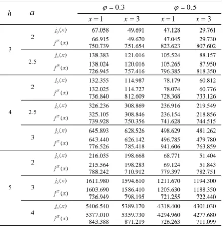
Table 2: Comparisons of values ARL₀ of j x₀( ) from explicit formulas with numerical approximations jIE( )x for

0 1

Z  and



positive.

h a 0.3 0.5

1

x x3 x1 x3

3 2

0( )

j x 67.058 49.691 47.128 29.761

( ) IE

j x 66.915 49.670 47.045 29.730 750.739 751.654 823.623 807.602

2.5

0( )

j x 138.383 121.016 105.524 88.157

( ) IE

j x 138.024 120.016 105.265 87.950 726.945 757.416 796.385 818.350

4 2

0( )

j x 132.355 114.987 78.179 60.812

( ) IE

j x 132.025 114.727 78.074 60.776 736.840 812.609 728.368 733.126

2.5

0( )

j x 326.236 308.869 236.916 219.549

( ) IE

j x 325.105 308.846 236.154 218.856 739.928 750.356 741.628 744.515

3

0( )

j x 645.893 628.526 498.629 481.262

( ) IE

j x 643.440 626.142 496.785 479.780 776.526 785.418 941.606 763.859

5 2

0( )

j x 216.035 198.668 68.771 51.404

( ) IE

j x 215.564 198.283 69.124 51.843 788.242 710.912 779.397 782.751

3

0( )

j x 1611.980 1594.610 1211.670 1194.300

( ) IE

j x 1603.690 1586.410 1205.630 1188.350 736.949 798.195 721.255 722.440

4

0( )

j x 5406.540 5389.170 4318.400 4301.030

( ) IE

j x 5377.010 5359.730 4294.960 4277.680 843.388 871.219 726.263 711.099

It can be seen from Tables 1 to 4, which the analytical explicit solutions are in good agreement with the results obtained from the numerical integral equation approach with 500 nodes in the integration rule. The computational times of the numerical integral equation approach take approximately 15 minutes while the results obtained from the explicit formula take less than 1 second which is much less than the former.

Table 3: Comparisons of values ARL₁ of j x₁( ) from explicit formulas with numerical approximations jIE( )x for

0 1, 2

Z   and



negative.

h a  0.5  0.3

1

x x3 x1 x3

3 2

1( )

j x 11.753 8.920 10.264 7.432

( ) IE

j x 11.742 8.913 10.256 7.427 740.942 745.279 766.870 768.726

2.5

1( )

j x 16.196 13.363 14.284 11.452

( ) IE

j x 16.178 13.350 14.270 11.441 740.194 739.179 754.686 752.439

4 2

1( )

j x 16.753 13.920 14.298 11.465

( ) IE

j x 16.734 13.907 14.284 11.457 742.455 745.794 760.162 761.768

2.5

1( )

j x 24.077 21.245 20.926 18.093

( ) IE

j x 24.044 21.217 20.899 18.072 740.818 739.227 750.677 753.172

3

1( )

j x 33.483 30.650 29.437 26.604

( ) IE

j x 33.431 30.604 29.393 26.565 742.721 744.752 761.675 769.959

5 2

1( )

j x 22.599 19.766 18.552 15.720

( ) IE

j x 22.572 19.764 18.536 15.710 742.222 743.922 746.512 751.129

3

1( )

j x 50.183 47.350 43.512 40.679

( ) IE

j x 50.088 47.262 43.433 40.607 744.983 743.532 757.572 801.813

4

1( )

j x 95.662 92.829 84.663 81.830

( ) IE

[image:4.595.321.531.437.660.2]

j x 95.452 92.626 84.481 81.655 743.860 763.422 763.328 760.832

Table 4: Comparisons of values ARL₁ of j x₁( ) from explicit formulas with numerical approximations jIE( )x for

0 1, 2

Z   and



positive.

h a 0.3 0.5

1

x x3 x1 x3

3 2

1( )

j x 6.596 3.763 5.598 2.765

( ) IE

j x 6.593 3.7464 5.597 2.768 809.333 776.635 776.713 778.242

2.5

1( )

j x 9.574 6.741 8.293 5.465

( ) IE

j x 9.567 6.738 8.287 5.458 739.632 743.673 739.227 740.635

4 2

1( )

j x 8.250 5.417 6.605 3.772

( ) IE

j x 8.248 5.421 6.606 3.779 881.608 879.081 862.904 867.459

2.5

1( )

j x 13.160 10.328 11.048 8.215

( ) IE

j x 13.149 10.321 11.040 8.213 796.993 773.781 747.635 752.091

3

1( )

j x 19.465 16.632 16.753 13.920

( ) IE

j x 19.441 16.613 16.734 13.906 761.207 756.636 763.312 768.524

5 2

1( )

j x 8.588 5.743 5.868 3.035

( ) IE

j x 8.589 5.763 5.884 3.058 755.091 758.664 753.641 754.203

3

1( )

j x 27.071 24.238 22.599 19.766

( ) IE

j x 27.033 24.207 22.572 19.747 753.282 783.609 755.341 755.201

4

1( )

j x 57.556 54.723 50.183 47.350

( ) IE

j x 54.442 54.616 50.088 47.262 840.331 846.633 756.340 753.501

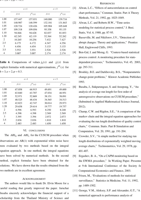
We also compare the values of j x0( ) and j x1( ) obtained from the explicit formulae and the numerical approximations for varying values of the parameter



. We assume that h3, a2 _{and the parameter of AR(1),}

[image:4.595.60.281.440.664.2]

[image:5.595.49.545.91.790.2]

Table 5: Comparisons of valuesj x₀( ) and j x₁( ) from explicit formulas with numerical approximationsjIE( )x for

3, 2, 0.3.

h a  

 x1 x3

( )

j x IE( )

j x j x( ) IE( )

j x

1.00 157.447 157.031 140.080 139.716

1.01 148.987 148.599 132.181 131.843

1.05 120.724 120.426 105.904 105.648

1.07 109.318 109.056 95.358 95.135

1.10 94.846 94.628 82.037 81.853

1.20 62.245 62.119 52.364 52.262

2 10.265 10.256 7.432 7.427

2.5 6.175 6.172 4.347 4.356

3 4.456 4.454 3.133 3.133

3.5 3.552 3.551 2.526 2.526

4 3.007 3.007 2.174 2.174

Table 6: Comparisons of valuesj x0( ) and j x1( ) from explicit formulas with numerical approximations,jIE( )x for

3, 2, 0.3.

h a 

 x1 x3

( )

j x IE( )

j x j x( ) IE( )

j x

1.00 67.058 66.915 49.691 49.600

1.01 63.840 63.707 47.034 46.951

1.05 52.971 52.869 38.151 38.091

1.07 48.525 48.434 34.565 34.513

1.10 42.823 42.747 30.014 29.973

1.20 29.658 29.614 19.777 19.757

2 6.596 6.593 8.250 8.248

2.5 4.398 4.398 2.569 2.569

3 3.395 3.394 2.072 2.073

3.5 2.836 2.836 1.810 1.810

4 2.483 2.483 1.650 1.650

VI. CONCLUSIONS

The ARL0 and ARL1 for the CUSUM procedure when observations are AR(1) with exponential white noise have been evaluated by two methods based on the integral equation approach. In one method, the integral equations have been solved by numerical methods. In the second method, explicit formulas have been obtained for the solutions. We have shown that the results obtained from the two methods are in excellent agreement.

ACKNOWLEDGMENT

The authors would like to thank Dr. Elvin Moore for a careful reading that greatly improved the paper. Jaruchat Busaba sincerely acknowledges the financial support of a

Technology and financial support for this research from King Mongkut’s University of Technology North Bangkok.

REFERENCES

[1] Alwan, L.C., “Effects of autocorrelation on control chart performance,” Commun. Statist. Part A Theory

Methods, Vol. 21, 1992, pp. 1025-1049. [2] Alwan, L.C. and Roberts H.W., “Time series

modeling for statistical process control,” J. Busi. Statis, Vol. 6, 1988, pp. 87-95.

[3] Basseville, M. and Nikiforov, I.V., “Detection of abrupt changes: Theory and applications,” Prentice Hall, Englewood Cliffs, 1993.

[4] Ben-Gal, I. and Morag, G. “Context-based statistical process control: A monitoring procedure for state- dependent processes,” Technometrics, Vol. 45, 2003, pp. 293-311.

[5] Brodsky, B.E. and Darkhovsky, B.S., “Nonparametric change-point problems,” Kluwer Academic Publisher, 1993.

[6] Busaba, J., Sukparungsee, S. and Areepong, Y., “An analysis of average run length for first order of autoregressive observations on CUSUM procedure,” (Submitted to Applied Mathematical Science Journal, 2012).

[7] Champ, C.W. and Rigdon, S.E., “A comparison of the markov chain and the integral equation approaches for evaluating the run length distribution of quality control charts,” Commun. Statis. Part B Simulation and Computation, Vol. 20, 1991, pp. 191-204.

[8] Crowder, S.V., “A simple method for studying run length distributions of exponentially weighted moving average charts,” Technometrics, Vol. 29, 1978, pp. 401-407.

[9] Ergashev, B. A., “On a CAPM monitoring based on the EWMA procedure,” In Working Paper. Presented at 9-th International Conference of the Society for Computational Economics and Finance, 2003.

[10] Frisen, M., “Evaluations of methods for statistical surveillance,” Statistics in Medicine, Vol. 11, 1992, pp. 1489-1502.

quickest change-point detection procedures,” Statistica Sinica, 2009.

[12] Golosnoy, V. and Schmid, W., “EWMA control charts for monitoring optimal portfolio weights,” Sequential Analysis, Vol. 26, 2006, pp. 195-224.

[13] Harris, T.J., and Ross, W.H., “Statistical process control procedure for correlated observations,” Canadian Journal of Chemical Engineering, Vol. 69, 1991, pp. 48-57.

[14] Hawkins, D.G. and Olwell, D.H., “Cumulative sum charts and charting for quality improvement,” New York: Springer, 1998.

[15] Hawkins, D.M., “A fast accurate approximation for average run lengths of CUSUM control charts,” J. Quality Technology, Vol. 24, 1992, pp. 37-43. [16] Knoth, S. and Schmid, W., “Control charts for time

series,” A review. In Frontiers in Statistical Quality Control (Edited by H.J.Lenze abd P’T’ Wilrich), Vol. 7, 2002, pp. 210-236.

[17] Lucas, J.M. and Saccucci, M.S., “Exponentially weighted moving average control schemes: properties and enhancements,” Technometrics, Vol.32, 1990, pp. 1-29.

[18] Mason, B. and Antony, J., “Statistical process control: an essential ingredient for improving service and manufacturing quality,” Managing Service Quality, Vol. 10, 2000, pp. 233-238.

[19] Mazalov, V.V. and Zhuravlev, D.N., “A method of Cumulative Sums in the problem of detection of traffic in computer networks,” Programming and Computer Software, Vol.28, 2002, pp. 342-348.

[20] Montgomery, D.C. and Mastrangelo, C.M., “Some statistical process control methods for autocorrelated data,” J. Quality Technol, Vol. 23, 1991, pp. 179-204. [21] Page, E.S., “Continuous Inspection Schemes,”

Biometrika, Vol.41, 1954, pp. 100-114.

[22] Robert, S.W., “Control chart tests based on geometric moving average,” Technometrics, Vol.1, 1959, pp. 239-250.

[23] Schmid, W and Rosolowski, M., “EWMA charts for monitoring the mean and autocovariances of stationary gausian processes,” Sequential Analysis, Vol. 22, 2003, pp. 257-285.

[24] Shewhart, A., “Economic control of quality of manufactured product,” New York: Van Nostrand, 1931.

[25] Sitter, R. R., Hanrahan, L., DeMets, D., and Anderson, H., “A monitoring system to detect increased rates of cancer incidence,” American Journal of Epidemiology, Vol.132, 1990, pp. 123-130.

[26] Sukparungsee, S. and Novikov, A.A., “On EWMA procedure for detection of a change in observations via martingale approach,” KMITL Science Journal: An International Journal of Science and Applied Science, Vol. 6, 2006, pp. 373-380.

[27] Sukparungsee, S. and Novikov, A.A., “Analytical approximations for detection of a change-point in case of light-tailed distributions,” Journal of Quality Measurement and Analysis, Vol. 4(2), 2008, pp. 49-56. [28] Woodall, W.H. and Adams, B.M., “The statistical

design of CUSUM charts,” Quality Engineering, Vol. 4, 1993, pp. 559-570.

[29] Wardell, D.G., Moskovitz, H and Plante, R.D., “Run distributions of special cause control charts for correlated processes,” Technometrics, Vol. 36, 1994, pp. 3-17.

[30] Woodal, W.H., and Faltin, F., “Autocorrelated data and SPC,” ASQC Statistics Division Newsletter, Vol. 13, 1993, pp. 18-21.

[31] Yashchin, E., “Performance of CUSUM control schemes for serially correlated observations,” Technometrics, Vol. 35, 1993, pp. 37-52.