Abstract— We derive explicit formulas for the average run
length (the first exit times) and the average of delay time on CUSUM procedure when observations are trend stationary first order of autoregressive (trend AR(1)) model with white noise exponential distribution by using an integral equation approach. Comparisons are made for the accuracy of results of the explicit formulas and the numerical approximations, which are in excellent agreement results. We also show that the computational times obtained from the explicit formulas are much less than the computational time obtained from the numerical approximations.
Index Terms— Trend Stationary First Order Autoregressive
Observation, Cumulative Sum, Average Run Length, Average of Delay Time
I. INTRODUCTION
raditionally, the observation of the Cumulative Sum (CUSUM) control chart, which was first introduced by Page in 1954, are normally and identically independent distributed random variables. In practice, this assumption is not always happen in real application such as in the continuous manufacturing processes where most observations are sequentially autocorrelated. Recently, many authors proposed new methods to investigate the CUSUM procedure when observation processes are autocorrelations for both case of stationary and non-stationary processes. In 1974, Johnson and Bagshaw [1] discussed the effect of autocorrelations on the performance of the cumulative sum (CUSUM) chart. In 1991, Harris and Ross [2] discussed the impact of autocorrelation on CUSUM and EWMA charts and pointed out that the average and the median run lengths of these charts were sensitive to presence of autocorrelation. Woodall and Faltin [3] have been discussed on the effect of autocorrelation on the performance of control charts and on how to deal with autocorrelation. Rao et al. [4] focused on the integral equation approach for computing the ARL for CUSUM control charts for AR(1) process. Karaoglan et al. Manuscript received April 17, 2012. This work was supported in financial by the Thailand Ministry of Science.
J. Busaba is with the King Mongkut’s University of Technology North Bangkok, Faculty of Applied Science, Department of Applied Statistics, Bangkok, Thailand, e-mail: [email protected]
S. Sukparungsee is with the King Mongkut’s University of Technology North Bangkok, Faculty of Applied Science, Department of Applied Statistics, Bangkok, Thailand, e-mail: [email protected]
Y. Areepong is with the King Mongkut’s University of Technology North Bangkok, Faculty of Applied Science, Department of Applied Statistics, Bangkok, Thailand, e-mail: [email protected]
[5] have discussed the performance comparison of residual control chart for trend stationary first order autoregressive processes. They applied the Shewhart, EWMA, CUSUM or GMA chart to the uncorrelated residuals. Busaba et al.[6] analyzed the average run length for AR(1) on CUSUM procedure by using Fredholm integral equation technique. Busaba et al.[7] have shown numerical approximations of ARL for AR(1) on Exponential CUSUM by using Gauss-Legendre rule. They obtained the results from the numerical integration method compared with results obtained from explicit formula which were in excellent agreement.
There are many characteristics to show the performance of procedure; such as Average Run Length (ARL) and the Average of Delay Time (AD). Both of them are frequently method used in procedure for evaluating the detection performance of various control charts. The expressions of them for the CUSUM and EWMA charts in detecting of mean shift in process, have been studied by [8], [9], [10], [11] and [12]. Various methods used to measure this performance of procedure; Monte Carlo Simulation (MC), Markov Chain Approach (MCA) (see [13]), Martingale Approaches (see [14, 15]) and Integral Equations (IE) (see [16], [17] and [18]). The first three methods give only closed-form formulas, while the last method gives the explicit formulae for the ARL and AD. Many authors have been derived the explicit form of ARL for the CUSUM (see [7], [19], [20], [21], [22], [23] and [24]). The proposed explicit expression is simple and easy to implement. In the present paper, the explicit formulae of ARL and AD on CUSUM procedure when observation processes are trend stationary first order autoregressive with exponential distributed white noise are proposed by using an integral equation approach, Fredholm second type integral equation. Next section describes the properties of CUSUM procedure. In section 3, the uniqueness of solution by using Banach’s fixed point theorem is described (see [25]). The solution for integral equation on CUSUM procedure for trend stationary first order autoregressive observations with exponential distributed white noise, based on the discussion of [19], [20] and [21, 22], is given in section 4. Comparison results are in section 5. Conclusions are pointed out in Section 6.
Analytical of ARL for Trend Stationary
First Order of Autoregressive Observations
on CUSUM Procedure
Jaruchat Busaba, Saowanit Sukparungsee, and Yupaporn Areepong
II. THE CUSUM PROCEDURE A. The Characteristics of CUSUM Procedure
The CUSUM chart, which we consider is under the assumption that sequential observations 1, 2,... are sequentially observed identically independent random variables with an exponential distribution function F x
, , where the parameter
has the value 0 in the in-control state (before a change-point time
), and this parameter 0changes to
(where 0) for out-of-control state. We assume that the parameters of the in-control and out-of-in-control states are known.According to the assumptions, F x
, is absolute continuous distribution with respect to F x
,0
. The alarm times for type of procedure for a statistic Xn typically defined as in equation (1) is
inf 0; ,
h n Xn h
(1)
whereh is a control limit on the value of Xn.
The statistical process control are required to measure of the average run length
ARL
which is the expectation of an alarm time( )
is taken to signal (wrongly) about a possible change. Ideally, an acceptable ARL of in-control process should be enough large and a small ARL when the process is out-of-control, so-called Average of Delay Time (AD) - the expectation of delay for true alarm time. Let
denote the expectation under distribution F x
,0
that the change-point occurs at point
. Typical measures for alarm times areh
ARL T (2) where T is given (usually large) and
1 .
h
AD (3)
TheARLand AD are two conflicting criteria that must be balanced in control charts.
B. The trend AR(1) on CUSUM Procedure
The CUSUM procedure is designed to detect an increase in the mean of an independent and identically distributed (i.i.d.) observed sequence of random variables 1, 2,...the recursive equation for CUSUM charts is defined as
1
n n n
X X Z a , n1, 2,... ,X0 x (4)
where Xn is the CUSUM value of a statistic after n observations, x is an initial value for Xn, y max 0,
y
and ais a constant. Mazalov and Zhuravlev [20] and George et. al [26] discussed many cases which lead to this recursive representation.
If the observations are trend stationary first order autoregressive (trend AR(1)) model with exponential distributed white noise as,
1
n n n
Z nZ ,
(5)
where n is the time of sampling, Zn is the sample value at
time n, is the constant, is the trend slope in terms of n , is the autoregressive coefficient
1 1
, and n isthe autoregressive white noise at time n following
exp .
n
Substitute Znfrom (5) into (4) then the CUSUM procedure can be written as
1 1 , 1, 2,... , 0 .
n n n n
X X nZ a n X x (6) III. UNIQUENESS OF SOLUTION TO AVERAGE RUN LENGTH
INTEGRAL EQUATION
Let X and X be the probability measure and the induced expectation corresponding to the initial value
0 .
X x Then it can be shown that the ARL for CUSUM at a given level (see [21] and [25]), defined as
x h,
j x
ARL
is a solution of the following integral equation
1 X
0 1
1 X
1 0
0 .j x I X h j X X j
(7) For the case,
nare exponential distributed observations have been proposed in [21, 22] and [23]. In this paper, we define
n are exponential distributed white noise with trend AR(1) observations by Zn
n
Zn1
nwhere
1
1
so (7) can be written as
0
0
0 1
1 0 , [0, ).
h
a x Z y
a x Z
j x e j y e dy
e j x a
(8) It is clear that solutions of the integral equation (8) are continuous functions, because the right hand side of (8) contains only continuous functions.
Recall that on the metric space of all continuous functions
, 1
, where
is a compact interval, and the norm defined as
,
x
j
Sup j x
the operator T is named a contraction if there exist a number
0
q
1
such that T j
1 T j2 q j1 j2 for allj j1, 2X. Now, define the operators T as
0
0
0 1
1 0
h
a x Z y
a x Z
T j x e j y e dy
e j
if x1.
(9) Then the integral equations in (8) can be written as
.T j x j x According to Banach’s Fixed Point
equation T j x
j x
has a unique solution (see [23]). To show the uniqueness of the solution of (8), we will prove in Theorem 3.1 that T is a contraction. Define the norms1
j
1
.
x
Sup j x
Theorem 3.1 On the metric spaces
1
1
,
the
operator T is a contraction. First, to show T is contraction we may check that for anyx1,and
j j
1,
2
1,
we have the inequality
1
2 1 2 11 ,
T j T j q j j where
q
is a positive constant,0
q
1
. According to (9) we have that
j
1T
j
2T
=Sup
j
x
=
0
1 2
0,
0 0 1 a x Z
x a
Sup j j e
0
1 2
0
h
a x Z y
e j y j y e dy
0
1 2 1
0,
0 0 1 a x Z
x a
Sup j j e
0
1 2 1
0
h
a x Z y
j j e e dy
=
0
1 2 1 0,
1
a x Z hx a
j
j
Sup
e
= 0
1 2 1
1
e
Z hj
j
=
q
1j
1
j
2 , where 0 1
1
1.
Z h
q
e
We have used the triangular inequality and the fact that,
1 2 1 2 1 2
0, )
0 0 .
x a
j j Sup j x j x j j
IV. APPROACH FOR INTEGRAL EQUATION OF TREND AR(1) OBSERVATIONS ON CUSUM PROCEDURE
A. The explicit formulae
In Theorem 4.1, we derive explicit solutions of the integral equations (8). The uniqueness of solutions is guaranteed by Theorem 3.1.
Theorem 4.1 The solution of (8) is
1 a Z0
h x, 0.j x e
h e e x (10)Proof.
0 0 0 11 0 , [0, )
h
a x Z y
a x Z
j x e j y e dy
e j x a
Define
0
.
h
y
d
j y e dy Now, we have
0 0 11 0 .
a x Z
a x Z
j x e d
e j (11) If x0 then j(0)
e
a Z0
d
.
Substitute j
0 into (10), we found that
01
a Z x.
j x
d
e
e
(12) Now the constantd can be found as
0
0 1
h
a Z y y
d
j
de e e dy
0
1 1 .
h
a Z
h h
e
e e he
Substitute the constant d into (12), we have
1 a Z0
h x, 0.j x e
h e e xThe explicit formula for the ARL and AD are presented as following
0
0 1 , 0
a Z h x
ARL j x e h e e x (13) and
0
1 1 , 0.
a Z h x
AD j x e h e e x (14) B. The numerical integral equation approach
The numerical scheme to evaluate solutions of the integral equations from section 4.1 is shown in the section. Firstly, the integral equation (8) can be written as follows:
0 0 0 1 0 , hj x j F a x Z
j y f a x Z y dy
(15) where F x
1 ex and f x
dF x
e x.dx
By Gauss-Legendre rule (See [16], [21], [22] and [27]) approximated the function
j x
as
1 0 0 1 1 IE mk k k i
k
j x j a F a x Z
w j a f a a a Z
(16) with kh w
m
and 1 .
2 k h a k m
V. COMPARISON RESULTS
All tables give a comparison of the approximated solutions ( )
IE
j x , the exact solutions j x( ), the absolute percentage difference
% ( ) ( ) 100%( )
IE
j x j x
Diff
j x
Table 1 and 3 show the computational times of approximately 10-15 minutes, by intel® Core™ i5 CPU with M540@ 2.53GHz processor, RAM 4.00 GB and 32-bit operation system, while the results obtained from the explicit formula take less than 1 seconds which is much less than the former.
The analytical explicit solutions are in good agreement with the results obtained from the numerical approximation with an absolute percentage difference less than 1% for 500 iterations of numerical integral approximation.
Table 1: Comparisons of values
ARL
andAD
ofj x
0( )
and
j x
1( )
from explicit formulae with numerical approximationsj
IE( )
x
for
0,
0. 2 . a
1,h 3
a
2,h 3
1
x x3 x1 x3
0.3 2 47.12781 29.7605 -0.3 2 121.13302 103.7650 47.04533
29.7301 120.8260 103.5110
910.96804
933.7130 937.6130 878.6290 0.17515
0.1021 0.2534 0.2448
2.5
105.5240 88.1565
2.5
227.5370 210.1700 105.2650 87.9496 226.9090 209.5940 917.0990 909.4550 822.2340 796.6810
0.2454 0.2347 0.2760 0.2741
2.9 178.5170 161.1500 2.9 360.5390 343.1720 178.2650 931.7630 160.7220 879.1900
359.5090 342.1940
795.0280 796.5410
0.1412 0.2656 0.2857 0.2850
0.5 2 30.8104 13.4432 -0.5 2 157.4470 140.0800 30.7774 13.4621 157.0310 139.7160 1027.5000 823.8100 807.6320 807.4770
0.1071 0.1406 0.2642 0.2599
2.5
78.6211 61.2538
2.5
287.4100 270.0430 78.4434 61.1282 286.6010 269.2860 807.1960 806.6970 804.0150 804.7620
0.2260 0.2050 0.2815 0.2803
2.9 138.3830 121.0160 2.9 449.8600 432.4920 138.0240 805.9640 120.7090 805.0120
448.5590 431.2440
805.5580 804.7310
0.2594 0.2537 0.2892 0.2886
0.7 2 17.4509 0.1437 -0.7 2 201.8030 184.4350 17.4552 0.1430 201.2520 183.9370 838.3180 806.8840 810.7530 808.1940
0.0246 0.4871 0.2730 0.2700
2.5
56.5015 39.2277
2.5
360.5390 343.1720 56.4839 39.1687 359.5090 342.0940 805.4170 804.2020 805.5890 804.4340
0.0311 0.1504 0.2857 0.3141
2.9 105.5240 88.1565 2.9 558.9560 541.5880 105.265 805.729 87.9496 804.0130
557.3250 540.0100
804.1690 803.9670
0.2454 0.2347 0.2918 0.2914
1
The average run length is from explicit formulae as in (13).
2The average run length is from explicit formulae as in (14). 3The average run length is from numerical integral equation as in (16). 4The absolute percentage difference.
5
[image:4.595.44.554.114.575.2] [image:4.595.41.297.653.758.2]CPU time used.
Table 2: Comparison of values j x0( ) and j x1( ) from explicit formulae with numerical approximations jIE( )x for
3, 2, 0.2, 0.25 . h a
x1 Diff(%)
3
x
(%) Diff ( )
j x IE( )
j x j x( ) IE( )
j x
1.00 51.7431 51.6467 0.1867 34.3758 34.3314 0.1293 1.01 49.3561 49.2661 0.1827 32.5499 32.5098 0.1233 1.05 41.2700 41.2009 0.1677 26.4501 26.4234 0.1010 1.07 37.9503 37.8895 0.1605 23.9902 23.9685 0.0905 1.10 33.6809 33.6301 0.1511 20.8718 20.8559 0.0762 1.20 23.7555 23.7263 0.1231 13.8740 13.8695 0.0324 2 5.8384 5.8363 0.0360 3.0054 3.0076 0.0731 3 3.1614 3.1609 0.0158 1.8387 1.8396 0.0489
Table 3: Comparisons of values
ARL
andAD
ofj x
0( )
and
j x
1( )
from explicit formulae with numerical approximationsj
IE( )
x
for
0,
0. 2 .
a
1,h 4
a
2,h 4
1
x x3 x1 x3
0.3 2 78.1792 60.8119 -0.3 2 279.3450 261.9780 78.0735 60.7756 278.4080 261.1100 821.2050 834.7610 998.0320 837.7100
0.1352 0.0597 0.3354 0.3313
3
498.6290 481.2620
3
1045.4500 1028.0900 496.7850 479.4870 1041.3500 1024.0500 928.3780 1152.1000 816.7590 803.7020
0.3698 0.3688 0.4013 0.4018
3.5 930.1200 912.7530 3.5 1831.6800 1814.3200 926.4930 1168.6000 909.1950 1164.9200
1824.3300 1807.0300
801.7350 829.1300
0.3899 0.3898 0.4013 0.4018
0.5 2 33.8241 16.4568 -0.5 2 378.0590 360.6920 33.9018 16.6039 376.7140 359.4160 841.7970 804.1070 830.9870 835.4940
0.2297 0.8939 0.3558 0.3538
3
378.0590 360.6920
3
1313.7900 1296.4200 376.7140 359.4160 1308.5700 1291.2800 803.3420 802.1110 801.5800 814.7150
0.3558 0.3538 0.3973 0.3965
3.5 731.3350 713.9630 3.5 2274.0900 2256.7200 728.5290 801.7670 711.2310 794.9660
2264.9000 2247.6100
798.8790 796.6030
0.3837 0.3827 0.4041 0.4037
0.7 2 103.9140 86.5464 -0.7 2 930.1200 912.7530 103.7020 86.4037 926.4930 909.1950 856.2590 801.5960 803.0460 802.7500
0.2040 0.1649 0.3899 0.3898
3
279.4080 261.9780
3
1641.5300 1624.1600 278.4080 261.1100 1634.9600 1617.6600 803.8880 800.6290 803.9830 804.4350
0.3579 0.3313 0.4002 0.4002
3.5 568.5820 551.2150 3.5 2814.4500 2797.0800 566.4490 799.3490 549.1510 801.0340
2803.0300 2785.7300
802.4690 825.0730
0.3751 0.3744 0.4058 0.4058
Table 4: Comparison of values j x0( ) and j x1( ) from
explicit formulae with numerical approximations IE( ) j x for 3, 2, 0.2, 0.25 .
h a
x1 Diff(%)
3
x
(%) Diff ( )
j x IE( )
j x j x( ) IE( )
j x
1.00 113.1330 112.8510 0.2499 95.7659 95.5358 0.2409 1.01 107.3050 107.0420 0.2457 90.4992 90.2856 0.2366 1.05 87.7453 87.5426 0.2315 72.9255 72.7651 0.2204 1.07 79.8073 79.6284 0.2247 65.8472 65.7073 0.2129 1.10 69.6900 69.5406 0.2148 56.8809 56.7664 0.2017 1.20 46.6697 46.5830 0.1861 36.7881 36.7261 0.1688 2 8.6013 8.5951 0.0721 5.7684 5.7664 0.0347 3 3.9879 3.9866 0.0326 2.6652 2.6652 0.0000 The results are showed in Table 2 and 4, we compare the value obtained from explicit formulae and numerical approximations for varying levels of the parameter of white noise,
.
We assume thath3,a2, 0.2and the parameter of AR(1),
0.25,0.25
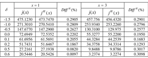
, respectively.Table 5: Comparison of values j x0( ) and j x1( ) from
explicit formulae with numerical approximations IE( ) j x for 1,h 3,a 2, 0, 0.25 .
x1 IE(%)
Diff
3
x
(%)
IE
Diff
( )
j x IE( )
j x j x( ) IE( )
j x
-1.5 475.1230 473.7470 0.2905 457.756 456.4320 0.2901 -1.0 271.3010 270.5410 0.2809 253.9340 253.2260 0.2796 -0.5 147.6770 147.2900 0.2627 130.3100 129.975 0.2577 0.0 72.6949 72.5352 0.2202 55.3277 55.2200 0.1950 0.1 61.6956 61.5691 0.2055 44.3284 44.2539 0.1683 0.2 51.7431 51.6467 0.1867 34.3758 34.3314 0.1293 0.5 27.2161 27.1938 0.0820 9.8488 9.8786 0.3017 0.6 20.5446 20.5426 0.0097 3.2374 3.2274 0.3098 Furthermore, we also compare these values for varying level of the parameter of trend slope
. We assume that1,h 3,a 2, 0
and 0.25 the results are showed in Table 5. The results are in good agreement with the numerical approximation with an absolute percentage difference less than 1% for 500 iterations.
VI. CONCLUSIONS
We derived analytically explicit formulas of ARL and AD on CUSUM procedure for the trend stationary first order autoregressive (trend AR(1)) observations with exponential distribution white noise. The accuracy of these explicit expressions are compared by numerical solutions of the integral equations based on using Gauss-Legendre integration rules. The numerical results and the values from the explicit formulas were in excellent agreement. The computation times required for the numerical computations were approximately 15 minutes compared with less than 1 second for the explicit formulas.
ACKNOWLEDGMENT
We would like to thank Dr. Elwin Moore for a critical proof-reading of the manuscript.
REFERENCES
[1] R.A. Johnson and M. Bagshaw, “The effect of serial correlation on the performance of CUSUM tests,” Technometrics, Vol. 16, 1974, pp. 103-112.
[2] T. J. Harris and W. H. Ross, “Statistical Process control procedure for correlated observations,” Canadian Journal of Chemical Engineering, Vol. 69, 1991, pp. 48-57.
[3] W.H. Woodal and F. Faltin, “Autocorrelated data and SPC,” ASQC Statistics Division Newsletter, Vol. 13, 1993, pp. 18-21.
[4] B.V. Rao, R.L. Disney and J.J. Pignatiello, “Uniqueness and converges of solutions to average run length integral equations for cumulative sum and other control charts,”IEEE Transactions, Vol. 33, 2001, pp. 463-469. [5] A.D Karaoglan and G.M. Bayhan, “Performance
comparison of residual control charts for trend stationary first order autoregressive processes,” Gazi university journal of science, Vol. 24, 2011, pp. 329-339.
[6] J. Busaba, S. Sukparungsee and Y. Areepong, “An analysis of average run length for first order of autoregressive observations on CUSUM procedure,”
(submitted for publication to Applied Mathematical Science Journal, 2012).
[7] J. Busaba, S. Sukparungsee and Y. Areepong, “Numerical Approximations of average run length for AR(1) on Exponential CUSUM,” (accepted to the
international multiconference of engineers and computer scientists 2012 (IMECS 2012) at Hong Kong, 2012).
[8] G. Lorden, “Procedures for reacting to a change in distribution,” Annual Mathematics Statistics, Vol. 42, 1971, pp. 1897-1908.
[9] H. M. Taylor, “A stopped Brownian motion formula,” Annual Probability, Vol. 3, 1975, pp. 234-246.
[10] M. Pallak and D. Siegmund, “A diffusion process and its application to detecting a change in the drift of Brownian motion,” Biometrika, Vol. 72, 1985, pp. 267-280.
[11]M. Pallak, “Average run lengths of an optimal method of detecting a change in distribution,” Annual statistics, Vol. 15, 1987, pp. 749-779.
[12] A.A. Novikov, “On the first passage time of an autoregressive process over a level and application to a disorder problem,” Theory of Probability and Its Applications, Vol.35, 1990, pp.269-279.
[13] J.M. Lucus and M. S. Saccucci, “Exponential weighted moving average control schemes: properties and enhancements,” Technometrics, Vol.32, 1990, pp.1-29. [14]S. Sukparungsee and A.A. Novikov, “On EWMA
procedure for detection of a change in observations via martingale approach,” KMITL Science Journal, An International Journal of Science and Applied Science, Vol. 6, 2006, pp. 373-380.
[15] S. Sukparungsee and A.A. Novikov, “Analytical approximations for detection of a change-point in case of light-tailed distributions,” Journal of Quality measurement and Analysis, Vol. 4, 2008, pp. 49-56. [16] S.V. Crowder, “A simple method for studying run
length distributions of exponentially weighted moving average charts,”Technometrics, Vol. 29, 1987, pp. 401-407.
[17]M. S. Srivastava and Y. Wu, “Evaluation of optimum weights and average run lengths in EWMA control schemes,” Communications in Statistics: Theory and Methods, Vol. 26, 1997, pp. 1253-1267.
[18] S. Knoth, “Accurate ARL calculation for EWMA control charts monitoring normal mean and variance simultaneously,” Sequential Analysis, Vol. 26, 2006, pp. 251-263.
[19]S. Vardeman and D. Ray, “Average Run Lengths for CUSUM schemes when observations are exponentially Distributed,” Technometrics, Vol. 27, 1985, pp. 145-150.
[20] V.V. Mazalov and D.N. Ahuravlev, “A method of Cumulative Sums in the problem of detection of traffic in computer networks,” Programming and Computer Software, Vol. 28, 2002, pp. 342-348.
[21] G. Mititelu, V.V. Mazalov and A. Novikov, “On CUSUM procedure for hyper-exponential distribution,” (submitted for publication to Statistics and Probability Letters, 2011).
East-West Journal of Mathematics, Special Vol., 2010, pp. 253-265.
[23]J. Busaba, S. Sukparungsee, Y. Areepong and G. Mititelu, “On CUSUM Procedure for Negative Exponential Distribution,” The 14th Conference of the ASMDA International Society, 2011, pp. 209-218. [24] J. Busaba, S. Sukparungsee, Y. Areepong and G.
Mititelu, “An analysis of average run length for CUSUM procedure with negative exponential data,” (accepted for publication to Chaing Mai Journal of Science, 2011.
[25] B.R. Venkateshwara, L. D. Ralph and J. P. Joseph, “Uniqueness and convergence of solutions to average run length integral equations for cumulative sums and other control charts,” IIE Transactions, Vol. 33, 2001, pp. 463-469.
[26] V. M. George, S. P. Aleksey and G. T. Alexander, “A Numerical Approach to Performance Analysis of Quickest Change-Point Detection Procedures,” Statistica Sinica, 2009 (in print).