Non Euclidean navigation

REVIEW

Non-Euclidean navigation

ABSTRACT

A basic set of navigation strategies supports navigational tasks ranging from homing to novel detours and shortcuts. To perform these last two tasks, it is generally thought that humans, mammals and perhaps some insects possess Euclidean cognitive maps, constructed on the basis of input from the path integration system. In this article, I review the rationale and behavioral evidence for this metric cognitive map hypothesis, and find it unpersuasive: in practice, there is little evidence for truly novel shortcuts in animals, and human performance is highly unreliable and biased by environmental features. I develop the alternative hypothesis that spatial knowledge is better characterized as a labeled graph: a network of paths between places augmented with local metric information. What distinguishes such a cognitive graph from a metric cognitive map is that this local information is not embedded in a global coordinate system, so spatial knowledge is often geometrically inconsistent. Human path integration appears to be better suited to piecewise measurements of path lengths and turn angles than to building a consistent map. In a series of experiments in immersive virtual reality, we tested human navigation in non-Euclidean environments and found that shortcuts manifest large violations of the metric postulates. The results are contrary to the Euclidean map hypothesis and support the cognitive graph hypothesis. Apparently Euclidean behavior, such as taking novel detours and approximate shortcuts, can be explained by the adaptive use of non-Euclidean strategies.

KEY WORDS: Cognitive map, Cognitive graph, Wayfinding, Path integration, Spatial cognition

Introduction

To go from one place to another involves the opening up of the vista ahead and closing in of the vista behind. When the vistas have been put in order by exploratory locomotion, the invariant structure of the habitat will be apprehended. One is oriented to the environment. It is not so much having a bird’s-eye view of the terrain as it is being

everywhere at once. (Gibson, 1979, p. 198)

In elegant research over the past half-century, a number of navigation strategies have been identified in species ranging from insects to humans that support a set of navigational tasks. Tasks include keeping track of where you are as you explore the environment, as in foraging; returning to a central place such as the home or nest, known as homing; traveling between familiar places by a known route; and traveling between familiar places by a new route or a novel shortcut. Navigational tasks can be distinguished from the online control of locomotion not by the scale of the distances involved but by the availability of perceptual

information about goals and barriers: whereas locomotor control

involves online guidance with respect to perceptible goals in‘vista

space’ (see Fajen and Warren, 2003; Zhao and Warren, 2017),

navigation involves wayfinding to goals beyond the sensory

horizon, in‘navigation space’(Meilinger et al., 2016). Navigation

thus entails some knowledge of the environment, however minimal. The question I pursue here is the nature of this knowledge.

A basic taxonomy of navigation strategies would include path integration, homing by beacons, piloting by landmarks, route navigation and map navigation (Gallistel, 1990; Trullier et al., 1997). Each strategy implicates a corresponding form of knowledge.

Let’s consider each in turn.

Path integration involves keeping track of one’s position and

orientation with respect to the starting or‘home’position, thereby

enabling a direct return path. Technically, path integration means sensing linear and rotational self-motion (e.g. via optic flow or vestibular information) and integrating to obtain displacements and turn angles, but the term normally includes information for the displacements and angles themselves (e.g. proprioception, celestial

compass). Some species appear to update a‘homing vector’that

specifies the distance and direction to home (Wehner, 2003), while others can remember the legs of the outbound path, at least up to a point (Wan et al., 2013). Path integration thus implies a simple vector memory, perhaps updated in working memory.

Homing by beacons takes advantage of perceptible features of the landscape that mark the home or goal location. An animal can navigate to a hidden goal by online steering toward visible beacons nearby (Collett, 1996). Beacons thus constitute visual information specifying the goal location, and could be acquired via perceptual learning.

Piloting by landmarks extends this strategy to recognizing configurations of landmarks, perhaps by matching the current vista with a remembered view (Cartwright and Collett, 1983; Morris, 1981). Piloting enables an animal to localize its current

position and orientation (take a‘fix’), to locate a goal by minimizing

the error between the current and remembered view, or to find home by associating a homing vector with particular landmarks or views (Cartwright and Collett, 1987). For this strategy, landmarks or views specifying known places must also be acquired through perceptual learning.

Route navigation builds on this ability by learning a sequence of places and corresponding actions, where places are identified by landmarks or views (Collett et al., 1998; Collett and Collett, 2002).

An animal with such ‘route knowledge’ can navigate between

familiar places by following a known sequence of place–action

associations. Confusion may ensue if two routes intersect at the same place, or the same route segment leads to two different places; this might be avoided by learning a route to each goal, or a sequence

of place–goal–action associations. While route knowledge allows

the navigator to repeat known paths between places, it is insufficient to generate novel paths or shortcuts.

Map navigation overcomes this limitation by relying on‘survey

knowledge’of the spatial positions of known locations in a common

coordinate system, akin to a cartographic map. Such a cognitive map

Department of Cognitive, Linguistic and Psychological Sciences, Brown University, Providence, RI 02912, USA.

*Author for correspondence ([email protected])

W.H.W., 0000-0003-4843-2315

Journal

of

Experimental

is the most general form of spatial knowledge and supports the most flexible navigation behavior, including novel routes and shortcuts. Although the term is often used rather loosely, I will follow the Euclidean definition common in the literature (see below), which has the virtue of clearly distinguishing map navigation from weaker strategies. While still hotly contested for honeybees (Cheeseman et al., 2014a, b; Cheung et al., 2014), it is generally believed that

rodents– and surely humans–possess metric cognitive maps of

their environments (Gallistel, 1990; Nadel, 2013).

The intuition that humans possess mental maps has a certain face validity. As we think about how to get from one place to another, it can

seem as if we are consulting an internal street map or a bird’s-eye view

of the terrain. But the metaphor of looking at a map in our own heads

commits the ‘representationalist fallacy’ that has long bedeviled

cognitive science (Huemer, 2001; Ramsey, 2007). If apprehending the environmental layout is explained as viewing an internal map (or, more generally, interpreting an internal representation), it implies an internal perceiver who is likewise viewing (or interpreting) its own internal map, leading to a regress. As Gibson (1979, p. 198) objected,

‘Way-finding is surely not the consulting of an internal map, for who

is the internal perceiver to look at the map?’. The intuition may

actually be a byproduct of our experience looking at cartographic maps, rather than playing a causal role in embedded navigation (Frankenstein et al., 2012). In my view, navigation theory should aim

to characterize what Gibson (1979) called‘apprehending the invariant

structure of the environment’, while avoiding the imputation of a

mental map read by the navigator.

If flexible navigation does not entail consulting a mental map,

what does it entail? How might an embedded navigator‘put vistas in

order by exploratory locomotion’ to apprehend ‘the invariant

structure of the habitat’? My working hypothesis is that the invariant

structure of pathways and barriers to locomotion is essentially topological, and can be characterized as a labeled graph. I suggest that apparently Euclidean behavior can be explained by the adaptive deployment of non-Euclidean navigation strategies.

The cognitive map hypothesis

Consider the cognitive map hypothesis and its rationale. The term was introduced by Tolman (1948) in a paper that played a pivotal role

in the turn from stimulus–response behaviorism to representational

cognitivism. Tolman (1948; p. 192) contrasted what he called a‘strip

map’, essentially a route to a goal, with a ‘comprehensive map’,

described as ‘something like a field map of the environment …

indicating routes and paths and environmental relationships’,

including places and extra-maze cues. Such a cognitive map would

explain an animal’s ability to take new routes, as well as Lashley’s

(1929) observation that a couple of rats climbed out of his maze and ran straight across the cover to a location directly above the food box.

It is this task of taking novel‘as-the-crow flies’shortcuts that is often

considered the raison d’etre of a metric cognitive map.

In their formative book, O’Keefe and Nadel (1978) made the case

for a Kantian conception of an absolute, unified space with a Euclidean geometric structure, and argued that cognitive maps of this space are necessary to account for flexible spatial behavior. Specifically, they argued that an allocentric Euclidean framework is a priori, and could not be induced from practical (e.g. embodied motor) experience. Much subsequent work has likewise assumed that cognitive maps have a metric Euclidean structure (Byrne et al., 2007; Gallistel, 1990; McNaughton et al., 2006), and Nadel (2013) recently affirmed this view.

Gallistel (1990) and Gallistel and Cramer (1996) described a specific procedure by which an animal could populate a metric map

by means of path integration. He assumed an allocentric Euclidean framework, including a Cartesian coordinate system with an origin at

home (xo,yo), a cardinaly-axis (‘North’) and an orthogonalx-axis. As

the animal leaves home, the path integrator registers displacements in

xandyto determine its current position vector (xa,ya) and its heading

angle (orientation) with respect to North. When the animal perceives a landmark at a particular egocentric bearing direction and

distance (egocentric vector), it computes the landmark’s allocentric

coordinates (xl,yl) via vector addition and enters it in the metric map.

As the navigator explores the environment, this process iterates,

building up a cognitive map of the terrain. The path integrator’s local

measurements of distance and direction are thus embedded in a globally consistent coordinate system, what roboticists call a global metric embedding. McNaughton et al. (2006) proposed a neural model of this map-building process, in which entorhinal grid cells define the coordinate system for a metric map that is reflected in hippocampal place fields (see also Bush et al., 2015; Moser et al., 2017).

As Gallistel (1990) points out, the advantage of a Euclidean map is that it preserves all geometric relationships between known places, including distances and angles. To find a shortcut between locations A and B, for example, one need only compute the direction and distance between their coordinates using trigonometry. This makes navigation highly flexible, for it supports novel paths, shortcuts and the integration of separately learned routes.

Behavioral evidence

Despite the compelling logic of Euclidean navigation, as an empirical matter the behavioral evidence for metric cognitive maps

is surprisingly weak, beginning with Tolman’s critical experiment.

Tolman et al. (1946) trained rats to a food box in a circuitous elevated maze. When the elevated maze was replaced by a sunburst alley maze with the trained path blocked, 36% of the animals took the most direct alley to the previous location of the food box (the rest were distributed among the 11 other alleys). It is seldom mentioned, however, that the location of the food box was marked with a lamp throughout the experiment! While the result may have provided

evidence of place learning rather than stimulus–response learning, it

was not evidence of a metric cognitive map. Today, we would say that this supposed shortcut behavior was actually a case of beacon

homing, and that Lashley’s (1929) anecdote probably involved

piloting by extra-maze cues.

History has repeated itself, as apparently Euclidean behavior has subsequently been explained by non-Euclidean strategies. Purported shortcuts in animals (e.g. Chapuis et al., 1987; Gould, 1986; Menzel et al., 2005) have been accounted for by beacon homing (Dyer, 1991; Foo et al., 2005; Wehner and Menzel, 1990), piloting by landmarks or familiar routes (Bennett, 1996; Collett and Collett, 2006; Dyer et al., 1993; Wehner et al., 1990). Explicit tests of metric maps in animals have routinely come up empty handed (Benhamou, 1996; Bennett, 1996; Gibson, 2001; Gibson and Kamil, 2001; Wehner et al., 1990).

In humans, experiments have demonstrated an ability to point in the direction of known locations in familiar or learned environments. This is often taken as evidence for a metric map. However, such directional estimates are highly unreliable, with

absolute (unsigned) errors of 20–100 deg and within-subject

angular standard deviations (AD) of 24–45 deg (Chrastil and

Warren, 2013; Foo et al., 2005; Ishikawa and Montello, 2006; Meilinger et al., 2014; Schinazi et al., 2013; Waller and Greenauer, 2007; Weisberg et al., 2014). If this ability governs navigation,

people would typically miss their destination by a wide berth.

Journal

of

Experimental

Moreover, humans have difficulty integrating separately learned routes, and between-route pointing is even more unreliable (Golledge et al., 1993; Ishikawa and Montello, 2006; Moeser, 1988; Schinazi et al., 2013; Weisberg et al., 2014). Nevertheless, such large errors are not enough to reject the metric hypothesis, for a cognitive map may be noisy, but still Euclidean.

Worse, explicit distance judgments (e.g. numeric estimates, marking a scale or paired comparisons of distances) are systematically biased by features of the landscape, such as the number of intervening junctions, turns, hills and boundaries (Byrne, 1979; Cohen et al., 1978; Kosslyn et al., 1974; McNamara, 1986; Sadalla and Magel, 1980; Sadalla and Staplin, 1980). Intersections tend to be orthogonalized to 90 deg (Byrne, 1979; Moar and Bower, 1983; Sadalla and Montello, 1989), yielding large distortions in cognitive maps (Golledge and Spector, 1978; Tversky, 1992). Nevertheless, such biases are also insufficient to reject the metric hypothesis, for even a distorted map can have an intrinsic Euclidean structure (Tobler, 1976). For example, when Golledge and Spector (1978) subjected paired comparisons of distances in an urban environment to multi-dimensional scaling, a technique that generates a Euclidean solution, they obtained a notably distorted map. Thus, a distorted cognitive map can still be Euclidean, even if it does not serve accurate navigation.

The metric postulates

The most serious challenge to the Euclidean hypothesis concerns

violations of the metric postulates (Beals et al., 1968). Thesine qua

nonof a metric space is a distance metric that satisfies the postulates

of: (a) positivity–the distance between point A and itself is zero,

and the distance between two points AB is greater than zero; (b)

symmetry– the distance AB is equal to the distance BA; (c) the

triangle inequality–for any three points, the sum of two sides AB

+BC is greater than or equal to the hypotenuse AC; and (d)

additivity–any two points A and C are joined by a segment along

which distances are additive, such that AC is the sum of AB and BC. A specifically Euclidean metric further requires that the triangle inequality satisfy the Pythagorean theorem.

There is empirical evidence that explicit distance estimates are asymmetric, such that judged distance from a landmark to a non-landmark is smaller than the reverse (Burroughs and Sadalla, 1979; Cadwallader, 1979; McNamara and Diwadkar, 1997; Moar and Carleton, 1982; Sadalla et al., 1980), apparently violating the symmetry postulate. It has been argued, however, that these results are due to biases during memory retrieval, rather than asymmetry in spatial knowledge itself (McNamara and Diwadkar, 1997; Newcombe et al., 1999). Intransitivity in distance estimates implies violations of additivity (Cadwallader, 1979), and orthogonalized

intersections imply violations of the triangle inequality (Byrne, 1979), but these postulates have not been directly tested.

Thus, the evidence for the Euclidean map hypothesis is not compelling, but neither is it decisively negative. In fact, it is unclear what sort of evidence could falsify the hypothesis, which counts as a strike against it. Given that there must be some error in a metric map, the degree of error or geometric inconsistency that would be sufficient to disconfirm the hypothesis is undefined. Comparative tests with alternative hypotheses may be more illuminating.

Maps and graphs

What’s the alternative? Modern geometry offers a spectrum of

conceptual possibilities for spatial structure that lie between mere route knowledge (Fig. 1A) and a full-blown Euclidean map (Fig. 1D). In his Erlangen program of 1872, Felix Klein (1893) addressed the 19th century crisis in mathematics by organizing the new geometries into a hierarchy, each defined by a group of transformations and the properties they leave invariant. The geometries range from strong, which preserve many properties, to weak, which preserve few: from Euclidean, to affine, to projective, to topology (Coxeter, 1961; Suppes, 1977). Gallistel (1990) evaluated their relative merits and concluded that animals must

possess Euclidean maps, but let’s reconsider some possible

descriptions of spatial knowledge.

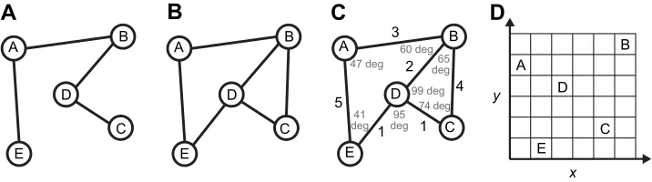
At the strong end of the spectrum lies a Euclidean map, which preserves distances and angles (and all the other properties) in a metric coordinate space (Fig. 1D). At the weak end of the spectrum lies topological spaces, which preserve neighborhoods, and topological structures such as graphs, which preserve adjacency. A topological graph of an environment consists of a network of nodes that might denote places, linked by edges that might denote

paths between them (Fig. 1B). Importantly, such a‘place graph’

captures the connectivity between places without embedding them in a coordinate system, and is thus coordinate free. Other types of

graphs are also possible, such as a‘view graph’in which nodes

denote specific views and edges denote the actions that relate them

(Gillner and Mallot, 1998), or a ‘neighborhood graph’ in which

nodes denote local regions and edges denote their adjacencies (see also Jacobs and Schenk, 2003; Kuipers et al., 2003; Mallot and Basten, 2009; Poucet, 1993).

Graph knowledge is richer than route knowledge (Fig. 1A), for a route may be a subgraph of a larger network (Fig. 1B). Whereas a route is a single chain of places and actions, a graph can capture multiple paths between two places, and multiple paths intersecting at one place. Thus, while route knowledge only supports travel along familiar paths, graph knowledge enables novel routes and detours by recombining edges in new sequences. This is illustrated

A B

D C E

A B

D C E

4 1 5

3

1 2

74 deg 41

deg 47 deg

60 deg 65 deg 99 deg

95 deg

y

x

A

B

D

C E

A

B

C

A B

D C E

D

Fig. 1. Alternative hypotheses for spatial knowledge.(A) Route knowledge: a line graph in which nodes denote places and edges correspond to actions. (B) Topological graph: a place graph in which nodes denote places and edges denote paths between them. (C) Labeled graph: a place graph with edge weights that denote approximate path lengths and node labels that denote approximate intersection angles. (D) Euclidean map: places correspond to coordinates

in a metric coordinate system. Modified from Warren et al. (2017).

Journal

of

Experimental

by perhaps the most well-known graph, the ‘tube map’ of the London Underground, which enables the user to travel between different locations by novel combinations of segments, despite its extreme topographic distortions.

Animal route networks have a graph-like quality. For example, Presotto et al. (2018) observed that capuchin monkeys frequently take

different branches at intersections they call‘change points’, which are

often proximal to resources and panoramic views. The monkeys thus appear to piece together different route segments depending on their current need for resources or visual information. At the neural level, hippocampal place fields are anchored to environmental features and their metric locations shift with transformations of the layout

(Dabaghian et al., 2014; Muller and Kubie, 1987; O’Keefe and

Burgess, 1996), leading some researchers to suggest that they reflect a topological graph (Dabaghian et al., 2012; Muller et al., 1996; Trullier and Meyer, 2000).

Graph knowledge has the advantage that available routes and detours are explicitly specified in a compact structure, whereas map knowledge requires that they be derived by additional operations on spatial coordinates. However, because a purely topological graph contains no metric distance and angle information, it cannot explain behavior such as taking the shortest detour or a novel shortcut. Given that humans can make at least rough direction and distance estimates, purely topological knowledge would appear to be inadequate.

The cognitive graph hypothesis

The most promising alternative, I believe, is an intermediate structure known as a labeled graph (Fig. 1C). This structure, which I

will call a‘cognitive graph’, is a place graph augmented by local

metric information, with edge weights denoting approximate path lengths, and node labels denoting approximate angles between adjacent paths at intersections. Importantly, this quantitative information is purely local, and is typically biased and imprecise, yielding spatial knowledge that is geometrically inconsistent. Nodes may also be labeled with other place information such as views,

landmarks, surface layout (local ‘geometry’) and functional

affordances, enabling self-localization and piloting (Epstein and Vass, 2014; Mallot and Basten, 2009).

A labeled graph is stronger than a topological graph but weaker than a Euclidean map. In contrast to a purely topological structure, it supports finding the shortest routes and detours through the graph; approximate shortcuts may even be estimated by vector addition along the shortest path to the goal. Their accuracy and precision, however, are limited by the local error in the graph. In contrast to a metric map, this local information is not embedded in a global coordinate system. Although such an embedding is theoretically possible (Hübner and Mallot, 2007), it presumes the Euclidean framework I am questioning here. Thus, what distinguishes a cognitive graph from a cognitive map is the absence of a global metric embedding, and hence a lack of geometric consistency.

Meilinger (2008) proposed a related ‘network of reference

frames’model, in which each vista has a local metric reference

frame, and these reference frames are linked together in a graph (see

also Poucet, 1993). Edges in the graph denote the‘perspective shift’

(translation and rotation) required to move between reference frames, but the local frames are not integrated into a common coordinate system. Shortcuts are generated by imagining a sequence

of perspective shifts from one’s current position to the goal location,

incrementally extending the local reference frame to include the goal. The main difference with cognitive graph theory is that the latter generates shortcuts by vector addition through a graph without requiring a common reference frame. Otherwise, the two

approaches agree that spatial knowledge need not be

geometrically consistent.

Building a cognitive graph

When exploring a new environment, a navigator could build a cognitive graph in a rather straightforward way. Local metric information is registered by the path integrator in idiothetic units (Chrastil and Warren, 2014a, 2017; Wittlinger et al., 2006). As the navigator path integrates from home, the home node is labeled with the direction of the departing path relative to local landmarks (or a celestial compass), path lengths are assigned to edge weights, and nodes are labeled with junction angles and other place information. New nodes are added as salient places and intersections are

encountered. These local measurements are not embedded in ana

prioriEuclidean framework, there is no coordinate system, nor is there a mechanism to check their geometric consistency.

Path integration, I would argue, is better suited to building a labeled graph than a geometrically consistent map. First, the human path integrator has poor resolution and systematic biases (Kearns et al., 2002; Loomis et al., 1993), and error accumulates with the length and number of legs of the journey (Wan et al., 2013). More importantly, path integration is not automatic and continuous, but intermittent and discontinuous. In an environment with stable visual landmarks for piloting, the path integrator actually shuts down, so the navigator is completely disoriented if landmarks unexpectedly vanish (Zhao and Warren, 2015a). Moreover, familiar visual landmarks act to reset the path integrator (both orientation and position) in humans (Mou and Zhang, 2014; Zhang and Mou, 2017; Zhao and Warren, 2015b) as in animals (Etienne et al., 2004; Knierim et al., 1998). Such a system is well suited for making local, piecewise measurements of rough travel distances and turn angles and registering them in a cognitive graph. If a familiar place is recognized, the path integrator is reset, the next leg of the journey is recorded, and the process iterates. The resulting graph labels may be noisy, biased by features of the landscape, and globally inconsistent. On this account, topological knowledge does not precede metric knowledge, as proposed by some early theorists (Piaget and Inhelder, 1967; Siegel and White, 1975); instead, the graph structure and local metric information are acquired together (Ishikawa and Montello, 2006). One would expect edge weights and node labels to become more accurate and precise with repeated exposure to an environment, but this does not indicate a qualitative shift from topological to Euclidean knowledge.

Shortcuts from graphs

Despite the geometric inconsistency of a cognitive graph, approximate shortcuts may be generated on the fly by vector addition along the shortest path through the graph. As proof of concept, note that vector addition can be performed in a coordinate-free space by application of the parallelogram law and cosine and sine rules (although this is not to claim that the brain performs this trigonometry). Such crude shortcuts may be sufficient to bring the navigator within sight of local beacons or landmarks, allowing them to home in on the goal. This adaptive combination of non-Euclidean strategies may explain successful shortcuts. Note that this process is

distinct from computing a single vector from one’s current

coordinates to the goal coordinates (e.g. Bush et al., 2015), and makes different predictions about pointing and shortcut errors.

We observed precisely this combination of strategies in a human version of the Gould/Dyer honeybee paradigm (Foo et al., 2005). In this paradigm, participants were first trained from the home location

to the locations of a red pole (A) and a blue pole (B), without walking

Journal

of

Experimental

the complete circuit. They were then displaced to home by wheelchair, guide-walked to A, and asked to walk a shortcut to the remembered location of B (and vice versa). Participants walked in a virtual reality laboratory (the VENLab) while wearing a head-mounted display, and their head position was recorded. The virtual environment (12×12 m) included a textured ground plane and the

poles. In a‘desert’environment with only the ground plane, the initial

walking direction was highly variable (AD=31 deg) and the final position error was large (equal to 47% of the straight-line distance). In

a‘forest’environment with a dense array of randomly colored poles,

the initial walking direction was somewhat less variable

(AD=24 deg) but the final position error was greatly reduced (only 11% of the straight-line distance). Importantly, trajectories often exhibited a mid-course correction as participants used the local configuration of colored poles to home in on the target location. Participants thus used a combination of a rough shortcut and piloting by landmarks. Unlike honeybees, however, the final approach to the target differed by an average of 53 deg from the trained approach, implying that humans are able to pilot by landmarks without exactly matching the views they experienced during learning.

Finally, with a cluster of seven colored poles surrounding the target location, participants made a direct shortcut, with precise initial directions (AD=5 deg) and small final errors (3% of the straight-line distance). Moreover, if the cluster was covertly shifted by 9 deg, shortcuts were completely captured by the cluster. In this

case, humans behaved much like Dyer’s (1991) honeybees, using

beacon homing to take an accurate shortcut. Apparently Euclidean behavior might be similarly explained by adaptive combinations of non-Euclidean strategies.

Routes or graphs?

To test whether humans learn a set of fixed routes or something closer to a network graph, we studied participants walking in a virtual hedge maze (11×12 m) (Chrastil and Warren, 2014b). They were instructed to freely explore the environment for 10 min and learn the locations of eight distinctive objects, while we tracked their movements (Fig. 2A). During the test phase, they were wheeled to a start object and asked to walk the shortest route to the remembered location of a target object within the maze corridors; crucially, on 40% of the trials the shortest route was blocked, forcing them to take a detour. Over half the trials were successfully completed within the allotted time. Importantly, of the successful trials, participants took novel routes on 63% of the direct trials and fully 90% of the detour

trials–that is, they took a path from the start object to the target

object that they had not travelled during exploration (Fig. 2B,C). Participants had thus not merely acquired route knowledge but had learned a graph of the environment, and were able to recombine segments in order to generate novel routes and detours.

Moreover, participants had also learned some local metric information. First of all, they took the shortest available route on 64% of the successful direct trials and 73% of the successful detour trials, far above the chance level. However, metric distance in the maze ( path length in meters) was correlated with topological distance (number of nodes or edges on the path). To dissociate them, we analyzed the five object pairs (out of a total of eight) in which the shortest route had at least one alternative route of the same topological length. Overall, participants took the metrically shortest route on 63% of successful trials, and the longer, topologically equivalent route on only 22%.

These results suggest that people learn more than route knowledge, and more than a topological graph, but knowledge consistent with a labeled graph that incorporates local information about path lengths. In similar experiments that manipulated the perceptual information available during learning, we found that vision alone is sufficient to acquire a topological graph (Chrastil and Warren, 2015), but podokinetic information is necessary to acquire metric properties (Chrastil and Warren, 2013, 2014b).

Graphs or maps?

In light of the animal and human literature reviewed above, the existing evidence appears inadequate to accept or reject the metric map hypothesis. Further demonstrations of unreliable or biased judgments in normal Euclidean environments are unlikely to be persuasive. We thus decided to approach the question from another direction: by creating matched Euclidean and non-Euclidean environments, we could dissociate the predictions of the metric map and cognitive graph hypotheses (Warren et al., 2017). We reasoned that, if the navigation system tries to build a metric map, participants would have greater difficulty learning the non-Euclidean environment because of its global inconsistency; however, if they were trained on the same configuration of objects in both environments, their shortcuts should be similar. In contrast, if navigators build a labeled graph, learning would be comparable in the two environments, but shortcuts in the non-Euclidean environment should be biased by the geometric discrepancies, in clear violation of the metric postulates.

s

A

B

C

s _s

b _b

b

Fig. 2. Route finding in a virtual hedge maze, for a representative subject.(A) Free exploration: all paths traveled during 10 min of exploration. s, sink; b, bookcase. (B) All paths leaving s or b during exploration; separate paths are represented in different colors. No continuous route was taken between them. (C) Test phase: a novel detour taken from s to b; yellow bar indicates blocked path. The participant had not traveled this route or the reverse during exploration (B), but generated it by recombining previously traveled segments (A), consistent with graph knowledge. Reproduced from Chrastil and Warren (2014a).

Journal

of

Experimental

Wormholes in virtual space

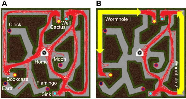
To compare the map and graph hypotheses, we created two versions of a virtual hedge maze (11×11 m) (Fig. 3). Both had a central home location that was linked by radial corridors to eight places marked by distinctive objects. The objects were only visible one at a time, so participants had to learn their locations by path integrating between

them. But the non-Euclidean maze contained two‘wormholes’that

covertly teleported the participant from one visual location to another and rotated them by 90 deg. This was accomplished by rotating the virtual environment 90 deg in the opposite direction when the participant walked through an invisible portal in a maze corridor. The wormhole entrance and exit views were matched so the transition was visually seamless.

Separate groups of participants learned the Wormhole maze and the Euclidean maze. A participant first explored the maze for 8 min, visiting each object at least once and passing through each wormhole at least twice (mean of 5.6 times). In the training phase, they were then trained to walk from home to each object until they could find the object within 30 s. This gave them experience with the same metric configuration of objects in both environments. We found that the number of trials to criterion was comparable in the two environments (the Bayes factor favored the null hypothesis by 3 to 1). Thus, the non-Euclidean environment was no more difficult to learn than the Euclidean environment, despite its global inconsistency.

In the test phase, we probed graph knowledge in half the participants by asking them to find routes between objects in the maze. On each trial, the participant walked from home to a specified start object, and was then told to walk to a target object within the

maze corridors. There were two pairs of ‘probe’ objects near a

wormhole entrance and exit, and two‘standard’pairs remote from

the wormholes. The results showed that both groups successfully learned the graph of the maze (Fig. 3). Moreover, the non-Euclidean group took good advantage of the wormholes, finding routes between the probe pairs that were half as long as those for the Euclidean group. Participants thus learned a labeled graph including local metric information.

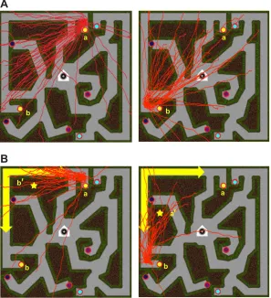
We probed survey knowledge in the other half of the participants by asking them to take novel shortcuts between the same pairs of objects. On each trial, the participant walked from home to a specified start object, the maze disappeared, and they were then told to turn and walk straight to the remembered location of a target object. The Euclidean group was quite accurate, for they walked in

the‘Euclidean direction’of the probe targets (defined by its trained

location with respect to home) with a mean constant error of only 4.4 deg (Fig. 4A). In contrast, the non-Euclidean group was

significantly biased in the‘wormhole direction’of the probe targets

(Fig. 4B), with a large constant error of 37.4 deg– close to the

expected error of 45 deg. Variable errors were characteristically large, but similar in both environments (mean within-subject AD of 27.5 deg in the Euclidean group, 30.4 deg in the non-Euclidean group), indicating comparable reliability. These results decisively supported the labeled graph hypothesis (the Bayes factor favored the graph model over the map model by more than 100 to 1). Essentially, participants learned the shortest way from one place to another, whether the environment was Euclidean or not.

Surprisingly, the participants were completely unaware of the wormholes. After spending an hour in the non-Euclidean maze, they failed to report any inconsistencies. Yet, their responses revealed large violations of the metric postulates in spatial knowledge. For example, referring to Fig. 4B, participants successfully walked from home to object a; but when they walked from home to object b and took a

shortcut to a, they went through the wormhole to location a′–6 m

distant from a! This represents a radical violation of the positivity postulate, for the reported distance between a and itself is much greater than zero. These responses also violate the triangle inequality, for the

hypotenuse ofΔHba is so large that the triangle is not closed. In a

second experiment, we even showed that participants acquire‘rips’

and‘folds’in their spatial knowledge of the wormhole maze, in which

the ordinal positions of objects are reversed (Warren et al., 2017). The results thus reveal a striking insensitivity to Euclidean structure.

Such findings are hard to explain under the cognitive map hypothesis. Perhaps an hour in the virtual maze was insufficient to learn a metric map, and with more experience participants would eventually do so. But this amount of exposure was sufficient for them to generate accurate shortcuts in the Euclidean maze, and variable errors in both mazes were comparable to previous results for familiar real environments. Or perhaps participants acquired a noisy metric map. That might account for the typically large variable errors, but it would not explain the systematic bias in the wormhole maze. What if the Euclidean group learned a metric map while the wormhole group learned a labeled graph? Yet, there is no evidence to support such different mechanisms, for the two groups had similar trials-to-criterion and short-cut variability. Moreover, because the non-Euclidean group failed to notice the wormholes, they could not have explicitly adopted a different learning strategy (see Warren et al., 2017, for more discussion).

Perhaps, if given sufficient information, participants would detect the geometric discrepancies and correct for the wormholes. In follow-up experiments with the wormhole maze, we (Ericson and Warren, 2010, 2012) added distal landmarks (four distinct towers visible from any point in the maze) and a sun that cast shadows in the maze. In one condition, these global cues were stationary, and

Sink

W

o

rmhole 2

A

B

Clock

CactusWell

Bookcase

Earth

Moon

Flamingo Home

Wormhole 1

Fig. 3. Route finding in the wormhole experiment. (A) Euclidean maze: all routes taken between the two pairs of probe objects (cactus_–bookcase, well_–sink). (B) Non-Euclidean maze, which contained two wormholes (yellow arrows): routes between the same probe objects took advantage of shorter wormhole paths on 84% of trials, compared with only 28% for the corresponding routes in A. Red traces represent all trials for all subjects. Reproduced from Warren et al. (2017).

Journal

of

Experimental

hence might reveal the maze rotation; in another, they rotated with the maze, undergoing large displacements that might be noticeable. In all conditions, however, we replicated our previous results: shortcuts were strongly biased in the wormhole direction.

What’s going on here? The cognitive graph hypothesis offers a

plausible interpretation of these findings. As one explores a new environment, the path integrator registers distances traveled and angles turned, and the navigation system builds piecewise a labeled graph of paths between salient places. These local measurements are noisy and biased, and drift over time. Consequently, landmarks for

familiar places are used to update the navigator’s location and reset

the path integrator. Suppose that a participant in the wormhole maze walks from home to object a, and home to object b, registering the path lengths and the angle between them (refer to Fig. 4B). If they then walk from b through the wormhole, the maze will rotate, and

they will pop out at a′–6 m away from a. In principle, this should be

sufficient to detect the discrepant locations of a and a′. But when the

navigator recognizes visual place a′ (‘Hello, a again!’), the path

integrator is reset, so the discrepancy is not detected and the wormhole goes unnoticed.

The resulting graph labels can thus be strongly biased by local experience and hence be geometrically inconsistent, with no global metric embedding. This would account for violations of the metric postulates. Geometrically inconsistent distance weights and angle labels yield violations of positivity and the triangle inequality. Paths that are learned in opposite directions may have different weights (a directed graph), yielding violations of the symmetry postulate. Euclidean and non-Euclidean environments are learned in the same manner, but the latter produce large discrepancies that are experimentally measurable.

The impossible heptagon

Recently, Marianne Strickrodt, Tobias Meilinger, Heinrich Bülthoff and I (unpublished) set out to test a strong prediction of the cognitive graph theory. The theory claims that shortcuts are generated by vector addition through a labeled graph. If labels in the graph are locally biased, shortcuts should be correspondingly biased. In contrast, cognitive map theory claims that shortcuts are generated by computing a vector from the current coordinates directly to the goal coordinates in a globally consistent map.

To test these predictions, we again created possible (Euclidean) and impossible (non-Euclidean) versions of a virtual maze (Fig. 5). In the possible maze, seven objects were positioned at the vertices of a regular heptagon, and participants walked in a zig-zagging corridor that visited all seven objects in a loop (Fig. 5A). In the impossible maze, however, the seven objects were mapped onto adjacent vertices of an expanded decagon (Fig. 5B). This created a large gap; when participants arrived at the terminal object (a book), they were seamlessly teleported over two empty vertices to a duplicate object (the book) by rotating the maze 108 deg.

The possible and impossible mazes were learned by two different groups of subjects. During the learning phase, they repeatedly walked three laps clockwise around the loop, followed by three laps counterclockwise, until they had memorized the sequence of seven objects. Going clockwise around the impossible maze, the objects were shifted outward and to the left compared with locations in the possible maze; going counter-clockwise, the objects were shifted outward and to the right. Thus, if participants built a labeled graph, the local information would be systematically biased and globally inconsistent. However, if they built a metric map, local clockwise and counter-clockwise measurements around a closed loop should

a a

a a

′

′

b b

b b

b

a

A

B

Fig. 4. Shortcuts in the wormhole experiment between cactus and bookcase.(A) Euclidean maze: all shortcuts from cactus (a) to bookcase (b) (left) and from b to a (right). (B) Wormhole maze: shortcuts are shifted in the‘wormhole direction’of the target (star at b′, left; or at a′, right). Reproduced from Warren et al. (2017).

Journal

of

Experimental

be embedded in a common coordinate system, minimizing error to achieve a globally consistent configuration; one would expect this process to yield a ring of equally spaced positions similar to the heptagon.

During the test phase, subjects performed a ‘pointing’task by

facing toward the remembered locations of target objects. On each trial, the participant was positioned at a start object and then asked to turn and face each of four target objects. The trick was that the four targets were tested in a clockwise order on half of the trials, and in a counter-clockwise order on the other half, thereby leading the participant through the graph in opposite directions. If participants estimate the target location by vector addition through a biased graph, the impossible group should make systematic errors when tested clockwise (outward to the left) and counter-clockwise (outward to the right), compared with the possible group.

That is precisely what we found. The possible group had constant errors close to zero, defined with respect to the heptagon target positions, so participants successfully learned the object locations. In contrast, the impossible group had significantly larger constant errors, which increased with target position around the loop. Specifically, when tested clockwise, pointing errors increased to the left, and when tested counter-clockwise, they increased to the right. For the first three targets in each direction, the constant error was close to the labeled graph prediction. But the error leveled off for the fourth target, perhaps as a consequence of partially averaging the clockwise path and the shorter counter-clockwise path, where it was the third target (and vice versa). For both groups, the within-subject variable error (s.d.) increased linearly with target number, consistent with the accumulation of error with vector addition through the graph, whereas the metric distance to the four targets increased non-linearly. Moreover, Meilinger et al. (2018) recently reported that the response time to point to a target also increases with the number of nodes through the graph.

In this simpler corridor environment, nearly half the participants reported noticing something unusual about the impossible maze, but their errors were not statistically different from those who did not notice. Overall, results for the impossible group very strongly supported the labeled graph theory (the Bayes factor favored the graph hypothesis over the map hypothesis by more than 50 to 1).

The impossible heptagon experiment thus confirms a specific prediction of cognitive graph theory, indicating that shortcuts are generated by a process of vector addition through a labeled graph.

Implications

The cognitive graph hypothesis may be able to account for a number of other observations in the literature. Consider, for example, the large individual differences that have been reported in survey tasks such as pointing between novel pairs of targets (Ishikawa and Montello, 2006; Weisberg and Newcombe, 2016; Weisberg et al., 2014). The large range of performance might be traceable to individual differences in path integration ability, and consequent variation in the precision of local metric information in a labeled graph. There may also be individual differences in the ability to perform vector addition in visual working memory, consistent with findings that differences in working memory (Weisberg and Newcombe, 2016) and perspective-taking ability (Wolbers and Hegarty, 2010) correlate with performance on survey tasks. Species differences in vector addition and visual working memory may even explain the paucity of evidence for novel shortcuts in insects and mammals (Meilinger, 2008).

Previous research has also consistently found that, when integrating two separately learned routes, pointing to a target on the same route (within-route) is more accurate than pointing to a target on the other route (between-route) (Golledge et al., 1993; Ishikawa and Montello, 2006; Schinazi et al., 2013; Weisberg et al., 2014). This falls right out of the cognitive graph theory, for on average there are fewer intervening nodes for within-route pointing than for between-route pointing, and hence the latter entails a greater accumulation of error. For example, in the environment tested by Weisberg et al. (2014), a back-of-the-envelope calculation reveals that within-route targets averaged 1.7 place nodes apart, whereas between-route targets averaged 2.8 place nodes apart. This might account for the significantly greater absolute error for between-route pointing than for within-route pointing. In contrast, pointing error did not correlate with the metric distance between targets, as might be expected for a Euclidean map.

In sum, the cognitive graph theory can potentially account for a range of behavioral data on route finding, novel detours, shortcuts

Book Book

Book

Key Key

Duck Duck

Comb

Comb

Dice Dice

Shoe _Shoe

Lamp _Lamp

A

B

Error

Fig. 5. The impossible heptagon experiment.Participants learn the locations of seven objects by walking around a zig-zag corridor in a loop. (A) Possible maze: the seven objects are positioned at the vertices of a heptagon. (B) Impossible maze: the same objects are positioned at seven adjacent vertices of a decagon; the participant is teleported over the gap to a duplicate object (book). When pointing from the current object (e.g. dice) to a target object (e.g. key), the target position in the impossible maze is expanded outward (dashed arrow) compared with the possible maze (solid arrow), yielding a predictable bias (dotted arrow).

Journal

of

Experimental

and pointing in both Euclidean and non-Euclidean environments. By tolerating geometric inconsistency, a labeled graph avoids the complications of building a metric map by embedding noisy, discrepant measurements in a globally consistent coordinate system. Nevertheless, the adaptive use of non-Euclidean strategies supports successful navigation, including the apparently Euclidean task of generating shortcuts on the fly. A cognitive graph, I suggest, thus

characterizes‘the invariant structure of the habitat’ that emerges

from‘putting vistas in order by exploratory locomotion’.

Acknowledgements

Thanks to Marianne Strickrodt, Tobias Meilinger, Elizabeth Chrastil, Jon Ericson, Mintao Zhao, Daniel Rothman and Ben Schnapp for their contributions to the research described in this article, and to Bob Shaw, from whom I learned to find the right geometry for your problem.

Competing interests

The author declares no competing or financial interests.

Funding

The research described in this article was supported by National Science Foundation (USA) grants BCS-0214383 and BCS-0843940.

References

Beals, R., Krantz, D. H. and Tversky, A.(1968). Foundations of multidimensional

scaling.Psychol. Rev.75, 127-142.

Benhamou, S.(1996). No evidence for cognitive mapping in rats.Anim. Behav.52,

201-212.

Bennett, A. T. D.(1996). Do animals have cognitive maps?J. Exp. Biol.199,

219-224.

Burroughs, W. J. and Sadalla, E. K.(1979). Asymmetries in distance cognition.

Geographical Analysis11, 414-421.

Bush, D., Barry, C., Manson, D. and Burgess, N.(2015). Using grid cells for

navigation.Neuron87, 507-520.

Byrne, R. W.(1979). Memory for urban geography.Q J. Exp. Psychol. (Colchester)

31, 147-154.

Byrne, P., Becker, S. and Burgess, N. (2007). Remembering the past and

imagining the future: a neural model of spatial memory and imagery.Psychol. Rev. 114, 340-375.

Cadwallader, M. T.(1979). Problems in cognitive distance: Implications for cognitive mapping.Environ. Behavior.11, 559-576.

Cartwright, B. A. and Collett, T. S.(1987). Landmark maps for honeybees.Biol.

Cybern.57, 85-93.

Cartwright, B. A. and Collett, T. S.(1983). Landmark learning in bees: experiments and models.J. Comp. Physiol. A151, 521-543.

Chapuis, N., Durup, M. and Thinus-Blanc, C.(1987). The role of exploratory

experience in a shortcut task by golden hamsters (Mesocricetus auratus).Anim. Learn. Behav.15, 174-178.

Cheeseman, J. F., Millar, C. D., Greggers, U., Lehmann, K., Pawley, M. D. M.,

Gallistel, C. R., Warman, G. R. Menzel, R.(2014a). Reply to Cheung et al.: the

cognitive map hypothesis remains the best interpretation of the data in honeybee navigation.Proc. Natl Acad. Sci. USA111, E4398.

Cheeseman, J. F., Millar, C. D., Greggers, U., Lehmann, K., Pawley, M. D. M., Gallistel, C. R., Warman, G. R. and Menzel, R.(2014b). Way-finding in displaced clock-shifted bees proves bees use a cognitive map.Proc. Natl Acad. Sci. USA 111, 8949-8954.

Cheung, A., Collett, M., Collett, T. S., Dewar, A., Dyer, F., Graham, P., Mangan,

M., Narendra, A., Philippides, A. and Stürzl, W.(2014). Still no convincing

evidence for cognitive map use by honeybees.Proc. Natl Acad. Sci. USA111, E4396-E4397.

Chrastil, E. R. and Warren, W. H.(2013). Active and passive spatial learning in

human navigation: acquisition of survey knowledge.J. Exp. Psychol. Learn. Mem. Cogn.39, 1520.

Chrastil, E. R. and Warren, W. H.(2014a). Does the human odometer use an

extrinsic or intrinsic metric?Atten. Percept. Psychophys.76, 230-246.

Chrastil, E. R. and Warren, W. H.(2014b). From cognitive maps to cognitive

graphs.PLoS ONE9, e112544.

Chrastil, E. R. and Warren, W. H.(2015). Active and passive spatial learning in

human navigation: acquisition of graph knowledge.J. Exp. Psychol. Learn. Mem. Cogn.41, 1162-1178.

Chrastil, E. R. and Warren, W. H.(2017). Rotational error in path integration:

encoding and execution errors in angle reproduction. Exp. Brain Res. 235, 1885-1897.

Cohen, R., Baldwin, L. M. and Sherman, R. C.(1978). Cognitive maps of a

naturalistic setting.Child Dev.1216-1218.

Collett, T. S.(1996). Insect navigation en route to a goal: Multiple strategies for the use of landmarks.J. Exp. Biol.199, 227-235.

Collett, T. S. and Collett, M.(2002). Memory use in insect visual navigation.Nat. Rev. Neurosci.3, 542.

Collett, M. and Collett, T. S.(2006). Insect navigation: no map at the end of the trail? Curr. Biol.16, R48-R51.

Collett, M., Collett, T. S., Bisch, S. and Wehner, R.(1998). Local and global

vectors in desert ant navigation.Nature394, 269.

Coxeter, F. R. S.(1961).Introduction to Geometry. New York: John Wiley.

Dabaghian, Y., Mémoli, F., Frank, L. M. and Carlsson, G.(2012). A topological

paradigm for hippocampal spatial map formation using persistent homology. PLoS Comput. Biol.8, e1002581.

Dabaghian, Y., Brandt, V. L. and Frank, L. M. (2014). Reconceiving the

hippocampal map as a topological template.Elife3, e03476.

Dyer, F.(1991). Bees acquire route-based memories but not cognitive maps in a

familiar landscape.Anim. Behav.41, 239-246.

Dyer, F. C., Berry, N. A. and Richard, A. S.(1993). Honey bee spatial memory: Use of route-based memories after displacement.Anim. Behav.45, 1028-1030.

Epstein, R. A. and Vass, L. K. (2014). Neural systems for landmark-based

wayfinding in humans.Philos. Trans. R. Soc. B369, 20120533.

Ericson, J. and Warren, W.(2010). The influence of external landmarks, the sun,

and cast shadows on learning a wormhole environment.J. Vis.10, 1057-1057.

Ericson, J. and Warren, W. H.(2012). The influence of cast shadows on learning a

non-Euclidean virtual hedge maze environment.J. Vis.12, 199-199.

Etienne, A. S., Maurer, R., Boulens, V., Levy, A. and Rowe, T.(2004). Resetting

the path integrator: a basic condition for route-based navigation.J. Exp. Biol.207, 1491-1508.

Fajen, B. R. and Warren, W. H.(2003). Behavioral dynamics of steering, obstacle

avoidance, and route selection.J.Exp. Psychol. Hum. Percept. Perform. 29, 343-362.

Foo, P., Warren, W. H., Duchon, A. and Tarr, M.(2005). Do humans integrate

routes into a cognitive map? Map- vs. landmark-based navigation of novel shortcuts.J. Exp. Psychol. Learn. Mem. Cogn.31, 195-215.

Frankenstein, J., Mohler, B. J., Bülthoff, H. H. and Meilinger, T.(2012). Is the map in our head oriented north?Psychol. Sci.23, 120-125.

Gallistel, C. R.(1990).The Organization of Learning. Cambridge, MA: The MIT

Press.

Gallistel, C. R. and Cramer, A. E.(1996). Computations on metric maps in

mammals: getting oriented and choosing a multi-destination route.J. Exp. Biol. 199, 211-217.

Gibson, J. J.(1979). The Ecological Approach to Visual Perception. Boston:

Houghton Mifflin.

Gibson, B. M.(2001). Cognitive maps not used by humans (Homo sapiens) during a

dynamic navigational task.J. Comp. Psychol.115, 397.

Gibson, B. M. and Kamil, A. C.(2001). Tests for cognitive mapping in Clark’s

nutcrackers (Nucifraga columbiana).J. Comp. Psychol.115, 403.

Gillner, S. and Mallot, H. A.(1998). Navigation and acquisition of spatial knowledge in a virtual maze.J. Cogn. Neurosci.10, 445-463.

Golledge, R. G. and Spector, A. N. (1978). Comprehending the urban

environment: theory and practice.Geographical Anal.10, 403-426.

Golledge, R. G., Ruggles, A. J., Pellegrino, J. W. and Gale, N. D.(1993).

Integrating route knowledge in an unfamiliar neighborhood: along and across route experiments.J. Environ. Psychol.13, 293-307.

Gould, J. L.(1986). The locale map of honey bees: do insects have cognitive maps? Science232, 861-863.

Hübner, W. and Mallot, H. A.(2007). Metric embedding of view graphs. A vision and odometry-based approach to cognitive mapping.Auton. Robots23, 183-196.

Huemer, M.(2001).Skepticism and the Veil of Perception. Lanham, MD: Rowman & Littlefield.

Ishikawa, T. and Montello, D. R.(2006). Spatial knowledge acquisition from direct experience in the environment: Individual differences in the development of metric knowledge and the integration of separately learned places.Cognit. Psychol.52, 93-129.

Jacobs, L. F. and Schenk, F.(2003). Unpacking the cognitive map: the parallel map theory of hippocampal function.Psychol. Rev.110, 285-315.

Kearns, M. J., Warren, W. H., Duchon, A. P. and Tarr, M. J. (2002). Path

integration from optic flow and body senses in a homing task.Perception31, 349-374.

Klein, F. (1893). A comparative review of recent researches in geometry

(Programme on entering the Philosophical Faculty and the Senate of the University of Erlangen in 1872).Bull. Am. Math. Soc.2, 215-249.

Knierim, J. J., Kudrimoti, H. S. and McNaughton, B. L.(1998). Interactions

between idiothetic cues and external landmarks in the control of place cells and head direction cells.J. Neurophysiol.80, 425-446.

Kosslyn, S. M., Pick, H. L. and Fariello, G. R.(1974). Cognitive maps in children and men.Child Dev.45, 707-716.

Kuipers, B., Tecuci, D. G. and Stankiewicz, B. J.(2003). The skeleton in the

cognitive map: a computational and empirical exploration.Environ. Behav.35,

81-106.

Journal

of

Experimental

Lashley, K. S.(1929).Brain Mechanisms and Intelligence. Chicago: University of Chicago Press.

Loomis, J. M., Klatzky, R. L., Golledge, R. G., Cicinelli, J. G., Pellegrino, J. W.

and Fry, P. A.(1993). Nonvisual navigation by blind and sighted: assessment of

path integration ability.J. Exp. Psychol. Gen.122, 73-91.

Mallot, H. A. and Basten, K.(2009). Embodied spatial cognition: biological and

artificial systems.Image Vis. Comput.27, 1658-1670.

McNamara, T. P. (1986). Mental representations of spatial relations. Cognit.

Psychol.87, 87-121.

McNamara, T. P. and Diwadkar, V. A.(1997). Symmetry and asymmetry of human

spatial memory.Cognit. Psychol.34, 160-190.

McNaughton, B. L., Battaglia, F. P., Jensen, O., Moser, E. I. and Moser, M.-B.

(2006). Path integration and the neural basis of the‘cognitive map’.Nat. Rev. Neurosci.7, 663-678.

Meilinger, T.(2008). The network of reference frames theory: a synthesis of graphs and cognitive maps. InSpatial Cognition VI(ed. C. Freksa, N. S. Newcombe, P. Gärdenfors and S. Wölfl), pp. 344-360. Berlin: Springer.

Meilinger, T., Riecke, B. E. and Bülthoff, H. H.(2014). Local and global reference frames for environmental spaces.Q. J. Exp. Psychol.67, 542-569.

Meilinger, T., Strickrodt, M. and Bülthoff, H. H.(2016). Qualitative differences in memory for vista and environmental spaces are caused by opaque borders, not movement or successive presentation.Cognition155, 77-95.

Meilinger, T., Strickrodt, M. and Bülthoff, H. H.(2018). Spatial survey estimation is incremental and relies on directed memory structures. In Spatial Cognition XI. 11th International Conference, Spatial Cognition 2018. Lecture Notes in Artificial Intelligence (Vol. 11034)(ed. S. Creem-Regehr J. Schöning and A. Klippel). Berlin, Heidelberg: Springer.

Menzel, R., Greggers, U., Smith, A., Berger, S., Brandt, R., Brunke, S., Bundrock, G., Hülse, S., Plümpe, T., Schaupp, F. et al. (2005). Honey bees navigate according to a map-like spatial memory.Proc. Natl Acad. Sci. USA102, 3040-3045.

Moar, I. and Bower, G. H.(1983). Inconsistency in spatial knowledge.Mem. Cognit. 11, 107-113.

Moar, I. and Carleton, L. R.(1982). Memory for routes. Q J. Exp. Psychol.

(Colchester)34A, 381-394.

Moeser, S. D.(1988). Cognitive mapping in a complex building.Environ. Behav.20, 21-49.

Morris, R. G.(1981). Spatial localization does not require the presence of local cues. Learn. Motiv.12, 239-260.

Moser, E. I., Moser, M.-B. and McNaughton, B. L.(2017). Spatial representation in the hippocampal formation: a history.Nat. Neurosci.20, 1448.

Mou, W. and Zhang, L.(2014). Dissociating position and heading estimations:

rotated visual orientation cues perceived after walking reset headings but not positions.Cognition133, 553-571.

Muller, R. U. and Kubie, J. L.(1987). The effects of changes in the environment on the spatial firing of hippocampal complex-spike cells.J. Neurosci.7, 1951-1968.

Muller, R. U., Stead, M. and Pach, J.(1996). The hippocampus as a cognitive

graph.J. Gen. Physiol.107, 663-694.

Nadel, L. E.(2013). Cognitive maps. InHandbook of Spatial Cognition(ed. D. E.

Waller and L. E. Nadel), pp. 155-171. Washington, D.C: American Psychological Association.

Newcombe, N., Huttenlocher, J., Sandberg, E., Lie, E. and Johnson, S.(1999).

What do misestimations and asymmetries in spatial judgement indicate about spatial representation?J. Exp. Psychol. Learn. Mem. Cognit.25, 986.

O’Keefe, J. and Burgess, N.(1996). Geometric determinants of the place fields of hippocampal neurons.Nature381, 425-428.

O’Keefe, J. and Nadel, L. E.(1978).The Hippocampus as a Cognitive Map. Oxford: Clarendon Press.

Piaget, J. and Inhelder, B.(1967).The Child’s Conception of Space. New York:

Norton.

Poucet, B.(1993). Spatial cognitive maps in animals: New hypotheses on their

structure and neural mechanisms.Psychol. Rev.100, 163-182.

Presotto, A., Verderane, M., Biondi, L., Mendonça-Furtado, O., Spagnoletti, N.,

Madden, M. and Izar, P. (2018). Intersection as key locations for bearded

capuchin monkeys (Sapajus libidinosus) traveling within a route network.Anim. Cogn.21, 393-405.

Ramsey, W. M.(2007).Representation Reconsidered. Cambridge: Cambridge

University Press.

Sadalla, E. K. and Magel, S. G.(1980). The perception of traversed distance.

Environ. Behav.12, 65-79.

Sadalla, E. K. and Montello, D. R.(1989). Remembering changes in direction.

Environ. Behav.21, 346-363.

Sadalla, E. K. and Staplin, L. J.(1980). The perception of traversed distance:

Intersections.Environ. Behav.12, 167-182.

Sadalla, E. K., Burroughs, W. J. and Staplin, L. J.(1980). Reference points in

spatial cognition.J. Exp. Psychol. Human Learn. Mem.6, 516-528.

Schinazi, V. R., Nardi, D., Newcombe, N. S., Shipley, T. F. and Epstein, R. A.

(2013). Hippocampal size predicts rapid learning of a cognitive map in humans. Hippocampus23, 515-528.

Siegel, A. W. and White, S. H.(1975). The development of spatial representations

of large-scale environments. InAdvances in Child Development, vol. 10 (ed. H. W. Reese), pp. 9-55. New York: Academic Press.

Suppes, P.(1977). Is visual space Euclidean?Synthese35, 397-421.

Tobler, W. R.(1976). The geometry of mental maps. InSpatial Choice and Spatial

Behavior(ed. R. G. Golledge and G. Rushton), pp. 69-82. Columbus, OH: Ohio State University Press.

Tolman, E. C.(1948). Cognitive maps in rats and men.Psychol. Rev.55, 189-208.

Tolman, E. C., Ritchie, B. F. and Kalish, D. (1946). Studies in spatial

learning. I. Orientation and the short-cut.J. Exp. Psychol.36, 13.

Trullier, O. and Meyer, J.-A.(2000). Animat navigation using a cognitive graph.

Biol. Cybern.83, 271-285.

Trullier, O., Wiener, S. I., Berthoz, A. and Meyer, J.-A.(1997). Biologically based artificial navigation systems: review and prospects.Prog. Neurobiol.51, 483-544.

Tversky, B.(1992). Distortions in cognitive maps.Geoforum23, 131-138.

Waller, D. and Greenauer, N.(2007). The role of body-based sensory information in the acquisition of enduring spatial representations.Psychol. Res.71, 322-332.

Wan, X., Wang, R. F. and Crowell, J. A.(2013). Effects of basic path properties on human path integration.Spat. Cogn. Comput.13, 79-101.

Warren, W. H., Rothman, D. B., Schnapp, B. H. and Ericson, J. D.(2017).

Wormholes in virtual space: from cognitive maps to cognitive graphs.Cognition 166, 152-163.

Wehner, R.(2003). Desert ant navigation: how miniature brains solve complex

tasks.J. Comp. Physiol. A189, 579-588.

Wehner, R. and Menzel, R.(1990). Do insects have cognitive maps?Annu. Rev.

Neurosci.13, 403-414.

Wehner, R., Bleuler, S., Nievergelt, C. and Shah, D.(1990). Bees navigate by

using vectors and routes rather than maps.Naturwissenschaften77, 479-482.

Weisberg, S. M. and Newcombe, N. S.(2016). How do (some) people make a

cognitive map? Routes, places, and working memory.J. Exp. Psychol. Learn. Mem. Cogn.42, 768.

Weisberg, S. M., Schinazi, V. R., Newcombe, N. S., Shipley, T. F. and Epstein, R. A.(2014). Variations in cognitive maps: Understanding individual differences in navigation.J. Exp. Psychol. Learn. Mem. Cogn.40, 669.

Wittlinger, M., Wehner, R. and Wolf, H.(2006). The ant odometer: stepping on stilts and stumps.Science312, 1965-1967.

Wolbers, T. and Hegarty, M.(2010). What determines our navigational abilities?

Trends Cogn. Sci.14, 138-146.

Zhang, L. and Mou, W.(2017). Piloting systems reset path integration systems

during position estimation.J. Exp. Psychol. Learn. Mem. Cogn.43, 472.

Zhao, M. and Warren, W. H.(2015a). Environmental stability modulates the role of

path integration in human navigation.Cognition142, 96-109.

Zhao, M. and Warren, W. H.(2015b). How you get there from here: Interaction of

visual landmarks and path integration in human navigation.Psychol. Sci.26, 915-924.

Zhao, H. and Warren, W. H.(2017). Intercepting a moving target: on-line or model-based control?J. Vis.17, 12-12.

Journal

of

Experimental