ISSN: 1816-949X © Medwell Journals, 2014
Corresponding Author: Ola Ragb, Department of Engineering Mathematics and Physics, Faculty of Engineering, Zagazig University, P.O. Box 44519, Zagazig, Egypt
Efficient Quadrature Solution for Composite Plate Problems
Ola Ragb, M.S. Matbuly and M. Nassar
1 1 2
Department of Engineering Mathematics and Physics, Faculty of Engineering,
1
Zagazig University, P.O. Box 44519, Zagazig, Egypt
Department of Engineering Mathematics and Physics, Faculty of Engineering,
2
Cairo University, Giza, Egypt
Abstract: The efficiency of different moving least square differential quadrature techniques are examined for
solving bending plate problems. Based on a transverse shear theory, the governing equations of the problem are derived. The transverse deflection and two rotations of the plate are independently obtained using moving least square approximations. The weighting coefficients for quadrature approximations are derived by three different techniques. For each one the accuracy and efficiency of the obtained results are examined. As well as the obtained results are compared with the previous analytical and numerical ones. Further, a parametric study is introduced to investigate the effects of elastic and geometric characteristics on the values of stress and transverse deflection of the plate.
Key words: Differential quadrature, irregular domains, composites, functionally graded, transverse shear theory
INTRODUCTION for solving plate problems. This method own the
Composite plates have been extensively preferred problems as well as irregular domains. Direct application materials in marine, mechanical, civil, nuclear and of MLSDQM go through some computational aerospace structures. Bending analysis for such complications with determination of partial derivatives of composites is one of the most important problems in the field quantities (Bui et al., 2011; Ragb et al., structural design. Due to the mathematical complexity of 2014). Later, Wen and Aliabadi (2008, 2012) proposed such problems, only limited cases can be solved two alternatives to overcome this difficulty. The first one analytically (Wang et al., 2001; Zenkour, 2003; indirectly evaluates second and higher order derivatives Timoshenko and Woinowsky-Krieger, 1959). Numerically, of the MLS shape functions at field points as much as finite difference, finite element, point collocation, first derivatives are obtained. The second proposal is to boundary element and discrete singular convolution apply MLS approximations over a finite difference grid methods have been widely applied for solving, such such that second and higher order derivatives, at the plate problems (Mukhopadhyay, 1989; Tu et al., 2010; interior nodes can be approximated using central finite Hrabok and Hrudey, 1984; Liew et al., 1998; Gupta et al., difference schemes.
1995; Tanaka et al., 1994; Tanaka and Bercin, 1998; The present research examins accuracy and efficiency
Civalek, 2007, 2009). of the earlier three mentioned MLSDQ techniques for
f y f y f G =Ge , Eγ =Ee , vγ =v
ik,i kj, j k i,i j, j
M +M =Q ,Q +Q = −q,(i=x, j=y),(k=x, y)
(
)
(
)
(
)
ii i,i j, j jj j, j i,i
ij i, j j,i
M D , M D ,
1
M D ,(i x, j y)
2
= − φ + νφ = − φ + νφ − ν
= − φ + νφ = =
(
)
i i i
Q =kGh w − ϕ , (i=x, y)
2 2 2 y x x 2 2 x y x
(1 ) (1 )
2 2 x y
x y w
D kGh 0
x (1 )
2 y x
∂ φ − ν ∂ φ + ν ∂ ϕ
+ + +
∂ ∂
∂ ∂
+ ∂ − ϕ =
∂ϕ ∂
∂ϕ − ν
γ +
∂ ∂
2 2 2
y y x
2 2
y x
(1 ) (1 )
2 2 x y
y x w
D kGh y 0
y
y x
∂ ϕ − ν ∂ ϕ + ν ∂ ϕ
+ + +
∂ ∂
∂ ∂
+ ∂ − ϕ =
∂ϕ ∂
∂ϕ
γ + ν
∂ ∂ 2 2 y y x y 2 2
w w w
kGh qe 0
y x y
x y
−γ
∂ϕ
∂ +∂ + γ∂ −∂ϕ − − γϕ + =
∂ ∂ ∂ ∂ ∂
(
ik i ik ij)
SS1 w=0, δ M + − δ(1 )M =0, (i=n, j=s, k=n,s)
(
ik j ik i)
SS2 w=0, δ ϕ + − δ(1 )M =0,(i=n, j=s, k=n,s)
(
ik j ik i)
w=0, δ ϕ + − δ ϕ =(1 ) 0,(i=n, j=s, k=n,s)
ik
1 i k 0 i k = δ = ≠
f f
ij ij
w(x,0 ) w (x, 0 ), M (x, 0 ) M (x,0 ), (i x, j x,y)
− = + − = +
= =
a parametric study is introduced to investigate the effects of elastic and geometric characteristic of the problem on the values of obtained results.
MATERIALS AND METHODS
Formulation of the problem: Consider a
non-homogeneous composite consisting of an isotropic plate bonded (along x-axis) to another one made of a FGM. The elastic characteristics of the composite vary such that:
(1) Where:
G = Shear modulus of the isotropic plate E = Young’s modulus of the isotropic plate v = Poisson’s ratio of the isotropic plate G = Shear modulus of the FG platef
E = Young’s modulus of the FG platef
v = Poisson's ratio of the FG platef
( = Constant characterizing the composite gradation Assume that the composite is subjected to a pure bending due to a laterally distributed load q (x, y ). Based on a first-order shear deformation theory, the equilibrium equations for such composite thin plate can be written as (Panc, 1975):
(2) Where:
M (i, j = x, y) = Bending and twisting moment resultantsij
Q (i = x, y)i = Shearing force resultants
The transverse deflection w (x, y) and the normal rotations nx (x, y), ny (x, y) are related to the moment and shear resultants through the following constitutive relations (Reddy, 1999):
(3)
(4)
where, D = Eh /12 (1-v ) and h are the Flexural rigidity and3 2
the thickness of the plate. The k is the shear correction factor which is to be taken 5/6 (Reddy, 1997, 1999). On suitable substitution from Eq. 3 and 4 into Eq. 2, the equilibrium equations can be written as:
(5)
(6)
(7) Where:
(… 0 = FG part
( = 0 = For isotropic one
According to the case of supporting, simply supported and clamped edge, the boundary conditions can be described as:
Simply supported: (8) (9) Clamped: (10) Where:
n = The subscripts represent the normal and tangent
s = The subscripts of the directions to the boundary edge
M , M and Q = Denote the normal bending moment,n ns n
twisting moment and shear force on the plate edge
nn and ns = The normal and tangent rotations about the plate edge
The continuity conditions (along the interface), must be also satisfied such that:
2 2 nn x xx x y xy y yy M =n M +2n n M +n M
2 2
ns x y xy x y yy xx M =(n −n )M +n n (M −M )
n x x y y Q =n Q +n Q
n nx x ny y ϕ = ϕ + ϕ
s nx y ny x ϕ = ϕ − ϕ
n
h j
i i i i i j i i
j 1 x y
( ) (x , y ) (x , y ) (x , y ) , ( w, , ), (i 1,N)
=
ρ = ρ ≅ ρ = φ ρ
ρ = ϕ ϕ =
∑
x m h T i i i 1u (x) P (x)a (x) P (x)a(x)
=
=
∑
=n
h 2
i i i
i 1 n
T 2
i i i
i 1
(a) (x - x )(u (x ) u )
(x - x )(P (x )a(x) u )
=
=
Π = ϖ − =
ϖ −
∑
∑
i x−x
A(x)a(x)=B(x)u
1
a(x)=A (x)B(x)u−
[
]
n
T T
i i i i i i
i 1 T
1 2 n
1 1 2
2 n n
A (x) P(x ) (x)P (x ) (x)P(x )P (x ),
u = u u u ,
(x)P(x ) (x) B(x) P(x) (x)
P(x )... (x)P(x )
=
= ϖ = ϖ
ϖ ϖ
= ϖ =
ϖ
∑
L
n
h T T 1
i i i
i 1
u (x) P (x)a(x) P (x)A (x)B(x ) u =− (x)u
=
= =
∑
φWhich means that the deflection and moments (along the interface) of isotropic and FG plates must be equaled.
Further, the force resultants and the rotations on the edge can be expressed in terms of the basic unknowns nx
and ny as follows (Reddy, 1999, 1997):
(12)
(13)
(14)
(15)
(16)
where, n and n are the direction cosines at a point on thex y
boundary edge.
Solution of the problem: The employed MLSDQ
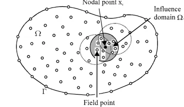
techniques can be summarized as follows: descretize the domain of the problem, S, into a finite number of nodes: {X = (x , y ), i = 1, N}. Each node is associated with threei i i
nodal unknowns (w, nx and ny). The influence domain for each node is determined as shown in Fig. 1. Over each influence domain, (S4, i = 1, N), the nodal unknowns can be approximated as Liew et al. (2002, 2003, 2004):
(17)
where, n is the number of nodes within the influence From which: domain, S4. The D = {w , nx, ny} approximate values for
h h h h
nodal unknowns w, nx and ny, respectively. The Nj (x , y )i i
is defined as the shape function of MLS approximation over the influence domain (S4, i = 1, N).
The nodal parameters: {w , i ni, ni} are always not
x y
equal to the physical values{w (x , y), i i nx (x , y ), i i ny (x , y )},i i
since the MLS shape functions Nj (x , y ) do not satisfy thei i
Kronecker delta condition generally. Apply the MLS technique to approximate u (x) to u (x) for any xh 0S such as (Lancaster and Salkauskas, 1981; Breitkopf et al., 2000):
(18)
where, a (x) = {a (x), a (x),... a (x)} is a vector of1 2 m T
unknown coefficients. The P (x) = {p (x), p (x),..., p (x)}T
1 2 m
[image:3.612.325.509.100.207.2]is a complete set of monomial basis. The m is the number
Fig. 1: Domain descretization for moving Least Squares Differential Quadrature Method
of basis terms. The coefficients a (x), (j = 1, m) can bej
obtained at any point x by minimizing the following weighted quadratic form:
(19)
Where:
n = Number of nodes in the neighborhood x and u = Nodal parameter of u (x)i
At point xi§i (x) = § (x-x ) is a positive weight functioni
which decreases as increases. It always takes unit value at the sampling point x and vanishes outside the domain of influence of x.
The stationary value of A (a) with respect to a (x) leads to a linear relation between the coefficient vector a(x) and the vector of fictitious nodal values u such as:
(20) (21) Where:
On suitable substitution from Eq. 21 into Eq. 19, u (x)h
can then be expressed in terms of the shape functions as:
(22)
( )
T( ) ( ) ( )
1 i x P x A x B xi−
φ =
( )
T( ) ( ) ( )
1 T( ) ( )
i x P x A x B xi x B xi
−
φ = = α
( ) ( )
( )
A x α x =P x
I I I
A(x)α(x)=P (x)−A (x) (x),(Iα =x,y)
IJ IJ IJ I J
J I
A(x) (x) P (x) A (x) (x) A (x) (x) A (x) (x), (I, J x, y)
α = − α − α −
α =
L T
j,L i j i j,L i j i
T
j i j,L i
(x ) c (x ) (x )B (x ) (x )B (x ), (L x, y)
φ = = α +
α =
LK T T
j,LK i j i j,LK i j i j i j,LK i
T T
j,L i j, K i j,K i j, L i
(x ) c (x ) (x )B (x ) (x )B (x ) (x )B (x ) (x )B (x ), (L, K x, y)
φ = = α + α +
α + α =
n L
L j i i,L i
i 1
(x) c (x ) (x) (L x, y)
=
ρ = =
∑
φ ρ =n LK
,LK j i i,LK i
i 1
n n
i,K i j,L j j
i 1 j 1
(x) c (x ) (x)
(x ) (x ) ,(L, K x,y)
=
= =
ρ = = φ ρ =
φ φ ρ =
∑
∑
∑
m
m
m
i 1j i 1j i 1j ij i 1j
,L i j ,LL i j 2
m
ij 1 ij 1 ij 1 ij ij 1
,K i j ,KK i j 2
m
i 1 j 1 i 1j 1 i 1j 1 i 1j 1 ,LK i j 2
x y
1 1
(x , y ) ( ), (x , y ) ( 2 ),
2h h
1 1
(x , y ) ( ), (x , y ) ( 2 ),
2h h
1
(x , y ) ( ),
4h
( w, , ), (L, K x, y)
+ − + −
+ − + −
+ + + − − − − +
ρ = ρ − ρ ρ = ρ − ρ + ρ
ρ = ρ − ρ ρ = ρ − ρ + ρ
ρ = ρ − ρ + ρ − ρ
ρ = ϕ ϕ = and (i, j 1,N)=
n
x j xx yy y j xy x j
ij ij ij ij ij x ij ij y
j 1
1 1 1 1
kGhc w D c c c kGh D c c 0,(i 1,N)
2 2 2 2
=
+ + − ν + − νγ − φ ϕ + + ν + − νγ ϕ = =
∑
n
y j xy x j yy xx y j
ij x ij ij y
ij ij ij ij
j 1
1 1
kGhc w D c c D c c c kGh 0,(i 1,N)
2 2
=
+ + ν + νγ ϕ + + − ν + γ − φ ϕ = =
∑
(23)
It should be noted that the MLS shape function and its derivatives are dependent on the weight function and the radius of influence domain. It’s also required that n$m in the domain of influence so that the matrix A (x) in Eq. 22 can be inverted (Reddy, 1999, 1997). Determine the MLS shape functions Nj (x , y ) and its partial derivativesi i
as proposed by Belytschko et al. (1996a, b) where: (24)
Since, A(x) is a symmetric matrix, then Eq. 24. For the partial derivatives of Nj (x , y ), (one can employ) yields:i i
(25)
Therefore, the problem of determination of the shape function is reduced to solution of Eq. 25. This Equation can be solved using LU decomposition and back-substitution which requires fewer computations than the inversion of A(x). The following techniques:
Direct technique: The first and second order partial
derivatives of Nj (x , y) can be determined as in Liew et al.i i
(2003): differentiate Eq. 26 with respect to I, J, (I, = x, y) such as:
(26)
(27)
The first and second order partial derivatives of the shape function can be described as:
(28)
(29)
Indirect technique: The first order partial derivatives of
[image:4.612.316.538.470.556.2]the shape function can be obtained as in Eq. 26 and 28, where:
Fig. 2: Grid descretization for the hybrid technique consisting of FDM and MLSDQM
(30)
The second order partial derivatives can be determined, using matrix multiplication approach (Shu, 2000) such that:
(31)
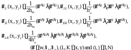
Finite difference technique: The first and second order
partial derivative of the shape function can be approximated over a finite difference grid (Wen and Aliabadi, 2012) with mesh side h as shown in Fig. 2.m
(32) A suitable linear interpolation must be applied to modify Eq. 32 for the intermediate points, (resulting from domain irregularities) as shown in Fig. 2.
On suitable substitution from Eq. 28-31 into the governing Eq. 5-7 the problem can be reduced to the following system of linear algebraic equations:
(33)
(
)
(
)
jn
xx yy y j x j y j ( y )
ij ij ij ij x ij ij y j 1
kGh c c c w c c c qe−γ , (i 1,N)
=
+ + γ − ϕ − + γ ϕ = − =
∑
(
)
(
)
(
)
(
)
(
)
m
i 1j i 1j i 1j i 1j ij 1 ij 1 ij ij 1 ij 1
m x x x x x x x
n
2 j i 1j 1 i 1j 1 i 1j 1 i 1j 1 i 1j i 1j
ij x y y y y y y
j 1
1 1 1
2h kGh w w 4D 2 1
2 2 2
1 1
4h kGh D D 0,(i 1,N)
2 2
+ − + − + − + −
+ + + − − − − + + −
=
− ν − ν − ν
− + ϕ + ϕ + ϕ + ϕ − + ϕ + γ ϕ − ϕ
+ ν − ν
−
∑
φ ϕ + ϕ − ϕ + ϕ − ϕ + γ ϕ − ϕ = =(
)
(
)
(
)
(
)
(
)
m
n ij 1 ij 1 i 1j 1 i 1j 1 i 1j 1 i 1j 1 i 1j i 1j 2 j
m x x x x x x ij y
j 1 i 1j i 1j ij 1 ij 1 ij ij 1 ij 1
y y y y y y y
1
2h kGh w w D D 4h kGh
2
1 1
4D 2 1 D 0, (i 1,N)
2 2
+ − + + + − − − − + + −
=
+ − + − + −
+ ν
− + ϕ − ϕ + ϕ − ϕ + νγ ϕ − ϕ − φ ϕ +
ϕ + ϕ + − ν ϕ + ϕ − + − νϕ + γ ϕ − ϕ = =
∑
(
) (
)
(
)
j
i 1j i 1j ij 1 ij 1 ij i 1j i 1j i 1j i 1j ij 1 ij 1
m x x y y
2 ( y ) n
j m
m ij y j 1
w w w w 4w w w 2h
4h qe
2h , (i, j 1,N)
kGh
+ − + − + − + − + −
−γ
=
+ + + − + γ − − ϕ − ϕ + ϕ − ϕ −
γ φ ϕ = −
∑
=(
)
(
)
(
x)
(
)
n
i 2 2 x y j 2 2 y x j
x y ij x y ij x x y ij x y ij y
j 1 n
2 2 y x j 2 2 x y j
x y ij y ij x x y ij x y ij y
j 1
SS1w 0, (n n )c (1 )n n c ( n n )c (1 )n n c 0,
1
D (n n )c 2n n c (n n )c 2n n c 0, (i 1,N)
2
=
=
= + ν + − ν ϕ + ν + + − ν ϕ =
− ν
− − − ϕ + − + ϕ = =
∑
∑
(
)
(
)
(
)
n
i j j
ij x y y x j 1
n
2 2 x y j 2 2 y x j
x y ij x y ij x x y ij x y ij y
j 1
SS2 w 0, n n 0,
(n n )c (1 )n n c ( n n )c (1 )n n c 0, (i 1,N)
=
=
= φ ϕ − ϕ =
+ ν + − ν ϕ + ν + + − ν ϕ = =
∑
∑
(
)
(
)
n n
i j j j j
ij x y y x ij x x y y
j 1 j 1
w 0, n n 0, n n 0, (i 1,N)
= =
=
∑
φ ϕ − ϕ =∑
φ ϕ + ϕ = =f f f
i i i i xx i i xx i i xy i i xy i i 1
w(x , y )=w (x , y ), M (x , y )=M (x , y ), M (x , y )=M (x , y ), (i=1, N )
2 2 i i 2 i i
exp( (d / c) ) exp( (r / c) )
d r
w (x) 1 exp( (r / c) )
0 d r
− − − ≤ = − − > 2 2
i i i
d = (x−x ) +(y−y )
(35)
Also on suitable substitution from Eq. 32 into the governing Eq. 5, 6, 7, the problem can be reduced to the following system of linear algebraic equations:
(36)
(37)
(38)
The boundary conditions can also be reduced to the following linear algebraic equations.
Simply supported:
(39)
(40)
Clamped:
(41)
Along, the interface the following algebraic equation must also be considered:
(42)
Where, N is the number of nodes along the interface.1
RESULTS AND DISCUSSION
For the present results, Gaussian weight function with a circular influence domain is adopted for the MLS approximation such as:
(43)
max m
r d
h =
m
h = 2β
s 4 2
ij ij ij ij
w=100wD /(qa ), M =10M /(qa ),σ = σ /E, (i, j=x,y)
s 4 2
ij ij ij ij
w=1600wD /(qa ), M =40M /(qa ),σ = σ /E,(i, j=x, y)
[image:6.612.108.266.93.191.2]ij ij w,M ,σ
Fig. 3: Skew rhombic plate
x to a field x in the influence domain of x . The r is thei i
radius of support domain and c is the dilation parameter In the present research, the dilation parameter is selected such as: c = r/4. Also, a scaling factor dmax is defined as:
(44)
where, h is the grid size which can be regarded as them
distance between the nodal point x and the secondi
nearest neighboring field nodes. For regular node arrangement spaced by $, h can be taken as:m
For squared plates, the numerical results are normalized such as Liew et al. (2003):
(45) As well as for skew rhombic plate shown in Fig. 3, the numerical results are normalized such as Liew et al. (2003):
(46) Where:
= Normalized deflection, moments and stresses a = Composite width
Ds = Flexural rigidity of the isotropic plate A numerical scheme is designed to investigate the influence of computational characteristics, (radius of support domain r, completeness order of the basis functions N and scaling factors dc max) on accuracy of the obtained results. The boundary conditions (28-31) are directly substituted into equilibrium ones (26 and 27). The reduced system is solved using MATLAB. The problem is solved over a regular grid with N = (7, 25). For different1
boundary conditions, Table 1 shows that the results for N = 11 are nearly the same, as those corresponding to1
N = (13, 25). Therefore, the parametric study is introduced1
[image:6.612.326.530.101.345.2]over grid 11×11 nodes.
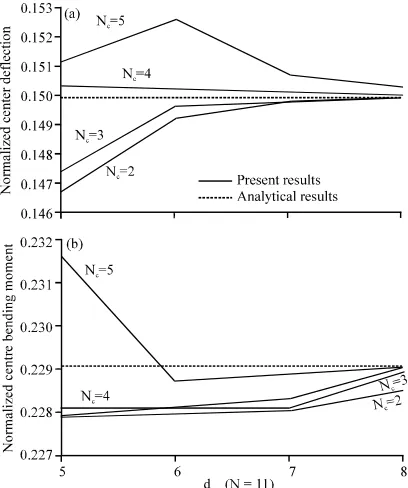
Fig. 4: Variation of the results with the radius of support domain and completeness order for a regular descretized clamped-clamped plate (N =1
11); (Redddy, 1999, 2002; Timoshenko and Woinowsky-Krieger, 1959)
Table 1: Comparison between the obtained bending moment and the previous analytical ones at the centre of a simply supported squared plate
No. of Obtained results (Support radius)
grid ---nodes Exact* r = 5.5 r = 6 r = 6.5 r = 7 6×6 0.47886 0.51503 0.520080 0.509190 0.49623 11×11 0.47886 0.47767 0.479290 0.477135 0.47845 16×16 0.47886 0.47902 0.476785 0.478440 0.47819 21×21 0.47886 0.47784 0.478620 0.478940 0.47786
Reddy (2002) and Timoshenko and Woinowsky-Krieger (1959)
*
Also, the completeness order N of the interpolationc
basis ranges from 2-7 with various scaling factors dmax
from 2-10 as shown Fig. 4-6. It is found that dmax$N +0.5 isc
required for reasonable numerical solutions. This was previously recorded by Liew et al. (2004). For irregular discretizations, the discrete nodes inside the plate are randomly generated while the boundary nodes are still equally spaced. For regular and irregular discretizations, Fig. 4-6 show that the accuracy of the obtained results increases with increasing both of N and the radius ofc
support domain while it decreases with increasing of the grid size h for different values of plate thickness h. Thism
result exactly agrees with that recorded in Liew and Han (1998).
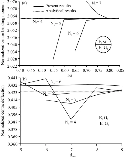
Figure 5 and 6 show that for irregular discretizations, To examine the validity of the obtained results, the one can select Nc$5 and d max$7 to obtain accurate
results.
Fig. 5: Variation of the results with the radius of support domain and completeness order for an irregular descretization simply supported plate; (Redddy, 1999; Timoshenko and Woinowsky-Krieger, 1959)
bending problem of regular and irregular isotropic plates is solved and compared with the previous analytical ones by Timoshenko and Woinowsky-Krieger (1959); Reddy (1999); Liew and Han (1997) and Sengupta (1995). Table 2-5 show a very good agreement between the obtained results and the previous analytical solutions. For clamped plates, the error between obtained results and the previous exact ones by Timoshenko and Woinowsky-Krieger (1959) and Reddy (1999) is #qa /D 104 G7. As well as Table 3-5 show that indirect moving least squares differential quadrature method is more efficient and accurate than the other DQ techniques.
Further, a parametric study is derived to investigate behavior of the composite due to Young's modulus gradation ratio (E /E ), shear modulus gradation ratio2 1
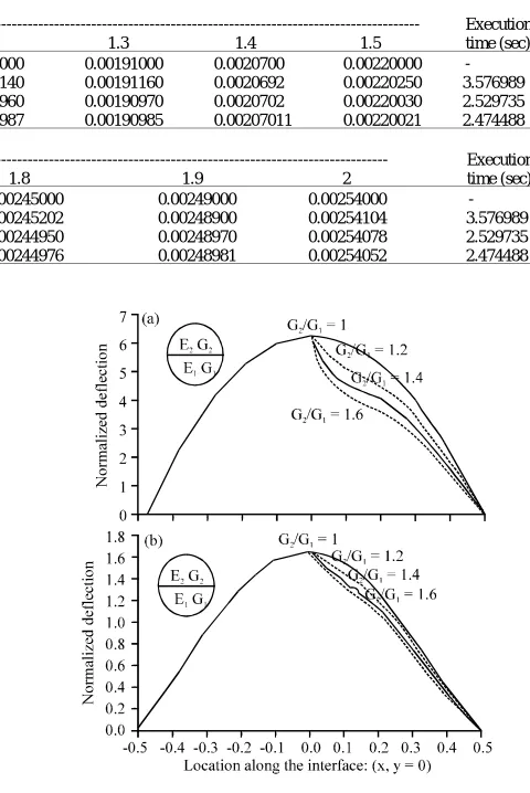
(G /G ), Poisson’s ratio (v /v ), graduation factor (2 1 2 1 (), stress distribution, Fyy, aspect ratio a/b and the interface location (a /a ) where a and b are the width and length of1 2
[image:7.612.133.488.377.696.2]the rectangular plate a = a +a . Figure 7-8 and 9 shows1 2
Table 2: Comparison between the obtained bending moment and the previous analytical ones at the centre of a clamped circular plate
Obtained results
---Support size Exact* N = 4 N = 5 N = 6 N = 7
c c c c
r = 0.7a 0.8125 0.8125 0.7301 0.8161 0.3536 r = 0.8a 0.8125 0.8125 0.8125 0.8124 0.8090 r = 0.9a 0.8125 0.8125 0.8125 0.8125 0.8111 r = a 0.8125 0.8125 0.8125 0.8125 0.8125 r = 1.1a 0.8125 0.8125 0.8125 0.8125 0.8125
Reddy (1999) and Timoshenko and Woinowsky-Krieger (1959)
*
Fig. 6: Variation of the results with the completeness order N and the number of grid points N for an irregularc 1
Table 3: Comparison between the obtained deflection by different methods and the previous analytical ones for simply supported skew rhombic plates at the centre (2 = 45°)
Exact MLSDQM MLSDQM+FDM IMLSDQM
--- --- --- ---Support size 1 2 N = 4c N = 5c N = 4c N = 5c N = 4c N = 5c
r = 0.5a 2.1193 2.1285 1.4257 1.7483 1.42575 1.74834 1.42592 1.75012 r = 0.6a 2.1193 2.1285 1.9384 1.9394 1.93843 1.93945 1.93884 1.94226 r = 0.7a 2.1193 2.1285 2.0541 2.0109 2.05412 2.01095 2.05495 2.01134 r = 0.8a 2.1193 2.1285 2.0888 2.0354 2.08884 2.03544 2.08888 2.03753 Execution time (sec) 4.317165 3.497017 3.237787
1 = Liew and Han (1997) and 2 = Sengupta (1995)
[image:8.612.296.536.296.655.2]Table 4: Comparison between the obtained deflection by different methods and the previous analytical ones for clamped circular plate at the centre Support size Exact* MLSDQM MLSDQM + FDM IMLSDQM r = 0.7a 1.6339 1.392360 1.392440 1.395200 r = 0.8a 1.6339 1.633900 1.633900 1.633900 r = 0.9a 1.6339 1.633900 1.633900 1.633900 r = a 1.6339 1.633900 1.633900 1.633900 r = 1.1a 1.6339 1.633900 1.633900 1.633900 Execution time (sec) 4.265994 3.245480 3.050844
Table 5: Comparison between the obtained deflection by different methods and the previous analytical ones, (*qa /D) for clamped rectangular plates at the centre4
b/a
--- Execution W (0,0) 1 1.1 1.2 1.3 1.4 1.5 time (sec) Exact* 0.00126000 0.00150000 0.00172000 0.00191000 0.0020700 0.00220000 -MLSDQM 0.00126100 0.00150040 0.00172140 0.00191160 0.0020692 0.00220250 3.576989 MLSDQM + FDM 0.00126054 0.00150028 0.00171960 0.00190970 0.0020702 0.00220030 2.529735 IMLSDQM 0.00126035 0.00150013 0.00171987 0.00190985 0.00207011 0.00220021 2.474488
b/a
--- Execution W (0,0) 1.6 1.7 1.8 1.9 2 time (sec) Exact* 0.002300000 0.00238000 0.00245000 0.00249000 0.00254000 -MLSDQM 0.002296000 0.00237800 0.00245202 0.00248900 0.00254104 3.576989 MLSDQM + FDM 0.002230100 0.00238030 0.00244950 0.00248970 0.00254078 2.529735 IMLSDQM 0.002230095 0.00238015 0.00244976 0.00248981 0.00254052 2.474488
Reddy (1999) and Timoshenko and Woinowsky-Krieger (1959)
[image:8.612.89.288.315.680.2]*
Fig. 7: Variation of the normalized deflection with supported; b) Clamped-clamped (E = E ; v = v ) Young's modulie for composite circular plates: a)
Simply supported; b) Clamped-clamped (G = G ;2 1 that the values of normalized deflection decrease with
v = v )2 1 increasing the Young’s modulus, the shear modulus and
Fig. 8: Variation of the normalized deflection with shear modulie for composite circular plates: a) Simply
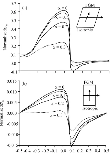
Fig. 9: Normalized deflection distribution through Fig. 11: Normalized stress distribution through different different locations for FG simply supported skew locations for FG; a) Simply supported; b) plate: a) ( = 1; b) ( = 10 Clamped-clamped (( = 10, h = 0.1)
Fig. 10: Variation of the normalized deflection with aspect ratio for composite rectangular plates: a) Simply supported; b) Clamped-clamped (E /E = 2;2 1
G = G ; v = v )2 1 2 1
the graduation factor (. While, these values increase with increasing of the aspect ratio (a/b) as shown in Fig. 10. Figure 11 show stress distribution, Fyy, through the
composite. This may be investigated through the stiffness concepts. Also, the computations declare that the results do not affect significantly by the Poisson’s ratio v , v .1 2
Further, Fig. 9 insist the advantages of FG composites that treat the interfacial discontinuity problems.
CONCLUSION
The efficiency and accuracy of moving least square differential quadrature techniques, are examined for solving composite plate problems. All of these methods lead to accurate results but indirect technique gives more the efficiency and accuracy. Also, a parametric study is introduced to investigate the effects of computational, geometric and elastic characteristics of the problem on the values of the obtained results. Further, this research can be considered as an extension for quadrature solutions of composite plate problems.
REFERENCES
[image:9.612.80.253.96.346.2] [image:9.612.97.261.399.610.2]Belytschko, T., Y. Krongauz, M. Fleming, D. Organ and Liew, K.M., C.M. Wang, Y. Xiang and S. Kitipornchai, W.K.S. Liu, 1996b. Smoothing and accelerated
computations in the element free Galerkin method. J. Computat. Applied Math., 74: 111-126.
Breitkopf, P., A. Rassineux, G. Touzot and P. Villon, 2000. Explicit form and efficient computation of MLS shape functions and their derivatives. Int. J. Numer. Methods Eng., 48: 451-466.
Bui, T.Q., M.N. Nguyen and C. Zhang, 2011. Buckling analysis of Reissner-Mindlin plates subjected to in-plane edge loads using a shear-locking-free and meshfree method. Eng. Anal. Boundary Elements, 35: 1038-1053.
Civalek, O., 2007. Three-dimensional vibration, buckling and bending analyses of thick rectangular plates based on discrete singular convolution method. Int. J. Mech. Sci., 49: 752-765.
Civalek, O., 2009. A four-node discrete singular convolution for geometric transformation and its application to numerical solution of vibration problem of arbitrary straight-sided quadrilateral plates. Applied Math. Modell., 33: 300-314.
Gupta, U.S., S.K. Jain and D. Jain, 1995. Method of collocation by derivatives in the study of axisymmetric vibrations of circular plates. Comput. Struct., 57: 841-845.
Hrabok, M.M. and T.M. Hrudey, 1984. A review and catalogue of plate bending finite elements. Comput. Struct., 19: 479-495.
Huang, Y.Q. and Q.S. Li, 2004. Bending and buckling analysis of antisymmetric laminates using the moving least square differential quadrature method. Comput. Meth. Applied Mech. Eng., 193: 3471-3492. Jafari, A.A. and S.A. Eftekhari, 2011. An efficient mixed
methodology for free vibration and buckling analysis of orthotropic rectangular plates. Applied Math. Comput., 218: 2670-2692.
Lancaster, P. and K. Salkauskas, 1981. Surfaces generated by moving least squares methods. Math. Comput., 37: 141-158.
Lanhe, W., W. Hongjun and W. Daobin, 2007. Dynamic stability analysis of FGM plates by the moving least squares differential quadrature method. Compos. Struct., 77: 383-394.
Liew, K.M. and J.B. Han, 1997. Bending analysis of simply supported shear deformable skew plates. J. Eng. Mech., 123: 214-221.
Liew, K.M. and J.B. Han, 1998. Bending solution for thick plates with quadrangular boundary. J. Eng. Mech., 124: 9-17.
Liew, K.M. and Y.Q. Huang, 2003. Bending and buckling of thick symmetric rectangular laminates using the moving least-squares differential quadrature method. Int. J. Mech. Sci., 45: 95-114.
1998. Vibration of Mindlin Plates-Programming the p-Version Ritz Method. Elsevier, New York. Liew, K.M., X. Zhao and A.J.M. Ferreira, 2011. A review
of meshless methods for laminated and functionally graded plates and shells. Compos. Struct., 93: 2031-2041.
Liew, K.M., Y.Q. Haung and J.N. Reddy, 2003. Moving least squares differential quadrature method and its application to the analysis of shear deformable plates. Int. J. Numer. Meth. Eng., 56: 2331-2351. Liew, K.M., Y.Q. Huang and J.N. Reddy, 2002. A hybrid
moving least squares and differential quadrature (MLSDQ) meshfree method. Int. J. Comput. Eng. Sci., 3: 1-12.
Liew, K.M., Y.Q. Huang and J.N. Reddy, 2004. Analysis of general shaped thin plates by the moving least-squares differential quadrature method. Finite Elements Anal. Des., 40: 1453-1474.
Mukhopadhyay, M., 1989. Vibration and stability analysis of stiffened plates by semi-analytic finite difference method, part I: Consideration of bending displacements only. J. Sound Vibrat., 130: 27-39. Panc, V., 1975. Theories of Elastic Plates. Springer Science
and Business Media, New York, USA., ISBN-13: 9789028601048, pp: 13-41.
Ragb, O., M.S. Matbuly and M. Nassar, 2014. Analysis of composite plates using moving least squares differential quadrature method. Applied Math. Comput., 238: 225-236.
Reddy, J.N., 1997. Mechanics of Laminated Composite Plates Theory and Analysis. CRC Press, Boca Raton. Reddy, J.N., 1999. Theory and Analysis of Elastic Plates.
Taylor and Francis, Philadelphia.
Reddy, J.N., 2002. Energy Principles and Variational Methods in Applied Mechanics. John Wiley and Sons, New York, USA.
Sengupta, D., 1995. Performance study of a simple finite element in the analysis of skew rhombic plates. Comput. Struct., 54: 1173-1182.
Shu, C., 2000. Differential Quadrature and its Application in Engineering. Springer, New York, ISBN-13: 9781852332099, Pages: 340.
Timoshenko, S. and S. Woinowsky-Krieger, 1959. Theory Wen, P.H. and M.H. Aliabadi, 2008. An improved of Plates and Shells. 2nd Edn., McGraw-Hill Book Co.,
New York, pp: 580.
Tu, T.M., L.N. Thach and T.H. Quoc, 2010. Finite element modeling for bending and vibration analysis of laminated and sandwich composite plates based on higher-order theory. Comput. Mater. Sci., 49: S390-S394.
Vanmaele, C., D. Vandepitte and W. Desmet, 2007. An efficient wave based prediction technique for plate bending vibrations. Comput. Meth. Applied Mech. Eng., 196: 3178-3189.
Wang, C.M., G.T. Lim, J.N. Reddy and K.H. Lee, 2001. Relationships between bending solutions of Reissner and Mindlin plate theories. Eng. Struct., 23: 838-849. Wang, X.W. and Z. Wu, 2013. Differential quadrature analysis of free vibration of rhombic plates with free edges. Applied Math. Comput., 225: 171-183.
meshless collocation method for elastostatic and elastodynamic problems. J. Commun. Numer. Meth. Eng., 24: 635-651.
Wen, P.H. and M.H. Aliabadi, 2012. A hybrid finite difference and moving least square method for elasticity problems. Eng. Anal. Boundary Elements, 36: 600-605.
Zenkour, A.M., 2003. Exact mixed-classical solutions for the bending analysis of shear deformable rectangular plates. Applied Math. Model., 27: 515-534.
Zhang, L.W., P. Zhu and K.M. Liew, 2014. Thermal buckling of functionally graded plates using a local Kriging meshless method. Compos. Struct., 108: 472-492.