Sensorless force feedback joystick control for teleoperation of construction equipment

warwick.ac.uk/lib-publications

Original citation:

Truong, Dinh Quang, Yoon, Jong II, Marco, James, Jennings, Paul A., Ahn, Kyoung Kwan and

Ha, Cheolkeun. (2017) Sensorless force feedback joystick control for teleoperation of

construction equipment. International Journal of Precision Engineering and Manufacturing,

18 (7). pp. 955-969.

Permanent WRAP URL:

http://wrap.warwick.ac.uk/88959

Copyright and reuse:

The Warwick Research Archive Portal (WRAP) makes this work by researchers of the

University of Warwick available open access under the following conditions. Copyright ©

and all moral rights to the version of the paper presented here belong to the individual

author(s) and/or other copyright owners. To the extent reasonable and practicable the

material made available in WRAP has been checked for eligibility before being made

available.

Copies of full items can be used for personal research or study, educational, or not-for profit

purposes without prior permission or charge. Provided that the authors, title and full

bibliographic details are credited, a hyperlink and/or URL is given for the original metadata

page and the content is not changed in any way.

Publisher’s statement:

“The final publication is available at Springer via

https://doi.org/10.1007/s12541-017-0113-5

”

A note on versions:

The version presented here may differ from the published version or, version of record, if

you wish to cite this item you are advised to consult the publisher’s version. Please see the

‘permanent WRAP url’ above for details on accessing the published version and note that

access may require a subscription.

© KSPE and Springer 2017

Sensorless Force Feedback Joystick Control for

Teleoperation of Construction Equipment

Truong Quang Dinh

_{, Jong Il Yoon}

_{, James Marco}

_{, Paul Jennings}

_{, Kyoung Kwan Ahn}

_{, and Cheolkeun Ha}

1 Warwick Manufacturing Group (WMG), University of Warwick, Coventry CV4 7AL, UK 2 Korea Construction Equipment Technology Institute, 36, Sandan-ro, Gunsan-si, Jeollabuk-do, 54004, South Korea 3 School of Mechanical Engineering, University of Ulsan, 93, Daehak-ro, Nam-gu, Ulsan, 44610, South Korea # Corresponding Author / E-mail: [email protected], TEL: +82-63-447-2552

KEYWORDS: Teleoperation, Force feedback, Neural network, Fuzzy, Sensorless

This paper aims to develop an innovative approach named sensorless force feedback joystick control for teleoperation of construction equipment. First, a force sensorless supervisory controller is designed with two advanced modules: a neural network-based environment classifier to estimate environment characteristics without requiring a force sensor and, a fuzzy-based force feedback tuner to generate properly a force reflection to the joystick. Second, two local robust adaptive controllers are simply built using neural network and Lyapunov stability condition to ensure desired task performances at both master and slave sites. A teleoperation system is setup to demonstrate the applicability of the proposed approach.

Manuscript received: November 9, 2016 / Revised: March 22, 2017 / Accepted: March 28, 2017

1. Introduction

Nowadays, teleoperation takes a key role in remote manipulation that allows users ability to perform naturally manual tasks at environments away from the normal human reach, such as undersea applications, hazardous assignments, minimally invasive surgical systems. In common, control schemes for teleoperation systems can be classified as either compliance control or bilateral control. In the compliance control,1-4 the contact force sensed by the slave device is not reflected back to the operator, but is used for the compliance control of the slave device. On the contrary, in the bilateral control,5-12 the contact force is reflected back to the operator. The operator is able to achieve physical perception of interactions at the remote site similar as directly working at this site. Consequently, it improves the accuracy and safety in the tele-operated manipulation. In addition, the force reflection can enhance the human operator’s task performance, for example in terms of task completion time, total contact time. Thus, the bilateral control has drawn a lot of attention.13,14

Two common architectures for a bilateral teleoperation system are known as: position-position and force-position architectures.7,13 In the first architecture, the master position is passed to the slave and the slave position is passed again to the master. Then, the reflected force applied to the operator is derived from the position difference between the two NOMENCLATURE

F_h = operator command

F_dr = desired reflected force

P_dr = desired reflected pressure

X_m = joystick shaft rotation

X_ds = slave desired movement

λ_p = conversion ratio between joystick and slave commands

u_s = slave controller output

X_s= slave actuation

F_e = loading force from environment

k_e = environment stiffness

c_e = environment damping coefficient

g_k = scaling factor of environment stiffness

g_c = scaling factor of environment damping coefficient

k_f = force feedback gain

λ_f = conversion ratio between F_dr and P_dr u_m = master controller output

ydesired = master/slave desired response

yactual = master/slave response

e = local controller control error

REGULAR PAPER

devices. However, this approach is not desirable in cases of free motion. In contrast, the force-position architecture uses directly the contact force measured at the remote site (using a force/torque/pressure sensor) to create an impact on the operator via a force feedback mechanism (FFM) with a force feedback gain (FFG). This method then provides the operator a better perception of tasks execution at the remote site. In the force-position architecture, besides precisely tracking control requirement, the selection of FFG greatly affects the task performance8. A large FFG results in a large reflected force and subsequently, could ensure a good task performance. However, this may cause the system to be unstable. Conversely, small reflected force leads to a poor sense for the operator. Many researches have been carried out to optimize the FFG. Raju proposed a two-port network model of a single degree of freedom remote manipulation system and applied it to design a force controller for transmitting the contact force information from a remote port to a local port. Kim15 suggested a control method as a combination of the bilateral control and compliance control to enlarge the FFG. However, these methods determined the FFG without considering dissimilar characteristics between different remote environments. To overcome that problem, several solutions were introduced. Kuchenbecker and Niemeyer9 introduced a force reflecting teleoperation with the use of model-based cancellation. Polushin and Lung10 proposed a projection-based force reflection algorithm for stable bilateral teleoperation. By using a high-gain input observer, the proposed algorithm eliminated the master motion induced by the reflected force without changing the human perception of the environment interactions. However, the authors did not consider the dynamic behaviors of the operator hand. Recently, Polushin and his colleagues11 developed a method named as generalized projection-based force reflection algorithm to solve the remained limitations in their previous studies. However, these suggested solutions were not proven in practical tests. Although the reported algorithms bring some remarkable results, there still remain some drawbacks such as: how to determine the FFG appropriately with environments containing unknown and uncertain characteristics and, it is difficult and expensive to attach proper sensors (force, torque or pressure sensors) to detect the environment conditions. Additionally, the sensors are easy to be damaged when the system operate in hazard conditions, especially for construction activities.

In order to deal with the above mentioned problems, the paper aims to develop a novel approach named sensorless force feedback joystick

control (SFFJC) for force-position bilateral teleoperation systems, specifically paying attention to construction equipment. This SFFJC is an advanced combination of a supervisory controller and two local master and slave controllers. First to drive sufficiently the force reflection, the force sensorless supervisory controller (FSSC) is designed with two main advanced modules: a neural network-based environment classifier (NNEC) and a fuzzy-based force feedback tuner (FFFT). Here, the NNEC takes part in estimating the environment characteristics without requiring a force (or torque or pressure) sensor and, the FFFT bases on the NNEC output and operator commands to generate a correspondingly FFG. Second, two local master and slave robust adaptive controllers (MRAC and SRAC, respectively) are simply built using neural network and Lyapunov stability condition to ensure that the manipulator tracks accurately any given trajectory while the FFM regulates exactly the desired force to provide the operator a better perception of task execution at the slave site. An experimental teleoperation system is setup to demonstrate the applicability of the proposed SFFJC approach.

The rest of this paper is organized as follows: Section 2 introduces the SFFJC control system concept and a simple teleoperation test rig; Section 3 describes procedure to design the FSSC while Section 4 shows the structures of the local controllers (MRAC and SRAC); the control validation process is carried out in Section 5 and, some conclusions are drawn in Section 6.

2. SFFJC Architecture and Test Rig Setup

2.1 SFFJC architecture

Furthermore, with the pneumatic solution, the FFM is able to work in safe conditions without damages from the operator.

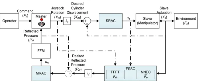
The proposed algorithm is composed of the three main routines: force sensorless supervisory controller and two local robust adaptive controllers. During the system operation, the human operator applies a force, Fh, to the joystick handle to provide a command for the slave. By this way, the joystick shaft rotation, Xm, is detected and converted into the slave command, X_ds, via a suitable ratio, λ_p. The SRAC attempts to make the slave execute the given command with high accuracy regardless any impact (unknown loading force) from the environment, F_e. Next, the command (u_s) and actual response (X_s) of the slave are acquired and input to the FSSC. This supervisory controller takes part in classifying the environment characteristics to estimate the loading condition at the slave site (Fe). Consequently, based on this estimated load value, the desired reflected force, Fdr, is properly produced. This resultant is converted approximately to a desired reflected pressure, Pdr, for the FFM using a transformed factor, λ_f. Finally, the MRAC drives the FFM (with command um) to create the desired pressure and, successively, creates the desired reflected force on the operator hand via the joystick handle. By this way, the operator can attain the truthful perception of the loading condition at the slave manipulator.

2.2 Teleoperation test rig

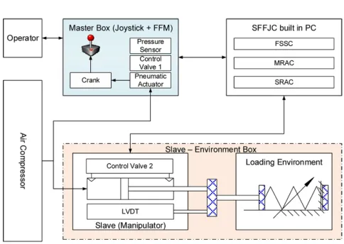
In order to evaluate the effectiveness of the SFFJC approach, a simple 1-DOF teleoperation test rig has been designed as Fig. 2. From this figure, the system consists of a master box, a slave – environment box in which a slave manipulator is connected to an environment simulator, and the SFFJC built in a personal computer (PC). The experimental system has been then fabricated as displayed in Fig. 3. In this study, only wired communication method is considered to develop the proposed control approach. To perform the wired communication between the SFFJC and the master/slave devices, a National Instrument (NI) multifunction data acquisition (DAQ) device with a suitable number of digital and analog channels is chosen.

As shown in Fig. 3(a), although two joysticks are installed in the master box, only one is used to develop the SFFJC while the other one will be used for the future research. The selected joystick is integrated with a FFM as described in Fig. 3(b). Rotation of the joystick handle generated by the human interaction is detected by a potentiometer attached at the pivot shaft of the joystick. This action is then converted into electrical commands to send to the SFFJC to drive the slave. For the force feedback concept as presented in the previous section, the FFM constructed by a mini pneumatic rotary actuator and two bias springs is attached to the opposite side of the joystick handle. Due to the limited free space of the joystick rotating mechanism, a slider-crank mechanism needs to be used to link the joystick rotating mechanism with the pneumatic rotary actuator. A proportional flow control valve (control valve 1) is used to drive the rotary actuator. And a pressure sensor is attached to the rotary actuator to perform the closed control loop and subsequently, to regulate any desired reflecting forces.

The slave – environment box setup is shown in Fig. 3(c) and Fig. 3(d). The slave employs an asymmetrically pneumatic cylinder as its manipulator. To perform the closed loop control, the cylinder is driven by another proportional control valve (control valve 2) and the piston displacement is measured by a linear variable displacement transducer

Fig. 2 Design layout for the teleoperation test rig

(LVDT). Moreover, second pressure sensor is attached to support the FSSC design. The environment simulator is presented by a spring-slider mechanism in which the spring stiffness and initial load can be manually adjusted (by changing the spring and the fixed position of the slider) to simulate different load conditions. An air compressor is installed as the main power source to supply the pressurized air for both the FFM and the slave cylinder. According to the design, the main components are properly chosen as listed in Table 1.

3. Force Sensorless Supervisory Controller

3.1 Supervisory control architecture

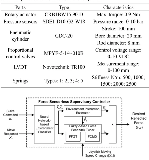
Configuration of the supervisory controller is described in Fig. 4. The FSSC consists of two main modules, NNEC and FFFT, with three inputs and one output. The first two inputs, the slave command (u_s) and its response (X_s), are received by the NNEC. Here, the classifier is built as a learning vector quantitative neural network (LVQNN) capable of detecting the working environment. Without loss of generality, the interactive environment can be represented by two factors: damping ce and stiffness ke. Thus, there are two outputs from the NNEC which are the predicted values of the environment damping and stiffness, and , respectively. These outputs are then fed into the environment interaction estimator to estimate the contact force between the manipulator and environment ( ). These outputs combined with another signal - joystick moving speed change ( ) are input to the FFFT module.

The FFFT module includes a fuzzy feedback gain tuner (FFGT) to tune the force feedback gain (k_f) based on the estimated damping and stiffness. Additionally, the impacts of the estimated contact force and

the human-joystick dynamics represented by the joystick moving speed change are taken into account for online refining the gain kf to ensure the stability performance of the mechanism. To fulfill this requirement, a fuzzy cognitive map-based decision (FCMD) tool is employed. The final output value of k_f is used to produce the desired force feedback (or desired reflect force, Fdr) which needs to be applied to the joystick.

3.2 Neural network-based environment classifier 3.2.1 Learning vector quantitative neural network

There exist many classification techniques successfully developed to support machine learning. Well-known techniques can be listed as logic-based algorithm as decision tree, support vector machines, static learning mechanism as Bayesian network, instance-based learning scheme as learning vector quantization (LVQ) or self-organizing map (SOM), and artificial intelligence-based method (fuzzy, genetic or neural network).16,17 Comparing to the others, intelligence-based methods offer higher adaptability and better performance in dealing with complex and partial unknown/unknown systems with limited and noisy data.16,17 Among intelligent solutions, neural network (NN) is realized as the powerful tool that provides higher flexibility and stronger capability than fuzzy logic while requires less computational effort than generic algorithm.17,18 Generally, neural network can be classified accordingly to the learning process: supervised and unsupervised learning. Supervised learning is training using desired responses for given stimuli while unsupervised learning is classification by “clustering of stimuli, without specified responses. However, these methods normally require a heavy training process. An LVQNN as depicted in Fig. 5 therefore is considered as feasible classification tool.

The LVQNN is a hybrid network which uses the advanced behaviors of both competitive learning networks and bases on the LVQ and Kohonen SOM to form the classification with the high speed. An LVQNN generally contains four layers: input layer with m nodes, first hidden layer named competitive layer with S1 nodes, second hidden layer named linear layer with S₂ nodes, and output layer with n nodes (in this case, S2 ≡ n).

The larger the hidden layer, the more clusters the competitive layer can learn, and the more complex mapping of input to target classes can be made19. With proper selection of the structure and training of the weighting factors, the LVQNN can classify any system information.

Each node, n_j, in the competitive layer is computed using the so-called nearest-neighbor method in which the Euclidean distance weight cˆ_e

kˆ_e

Fˆ_e=k_eX_s+c_eX·_s

X··_m Table 1 Specifications of the system components

Parts Type Characteristics

Rotary actuator CRB1BW15 90-D Max. torque: 0.9 Nm Pressure sensors SDE1-D10-G2-W18 Pressure range: 0-10 bar

Pneumatic

cylinder CDC-20

Stroke: 100 mm Bore diameter: 20 mm

Rod diameter: 8 mm Proportional

control valves MPYE-5-1/4-010B

Control voltage range: 0-10 VDC

LVDT Novotechnik TR100 Measurement range: 0-100 mm

Springs Types: 1; 2; 3; 4; 5 Stiffness N/m: 500; 1000; 1500; 2000; 2500

Fig. 4 Configuration of supervisory controller

function, D, is employed:

(1)

where X is the input vector; W1(j,i) is the weight of node jth in the

competitive layer corresponding to element ith of the input vector. Next, the derived Euclidean distances are fed into function C which is a competitive transfer function. This function returns an output vector o1, with 1, where the net input vector reaches its maximum value, and

0 elsewhere. The achieved output vector is then input to the linear layer to produce a vector o2, where each element can be computed as

(2)

where W2(k,j) is the weight of node kth in the linear layer corresponding

to element jth of the competitive output vector; k_W(k) is the linearized gain of node kth in the linear layer.

In the learning process, the weights of LVQNN are updated by the well-known Kohonen rule as

(3)

where μ is the positive learning ratio and is decreased with respect to the number of training iterations (niteration), μ=niteration.

3.2.2 LVQNN design for NNEC

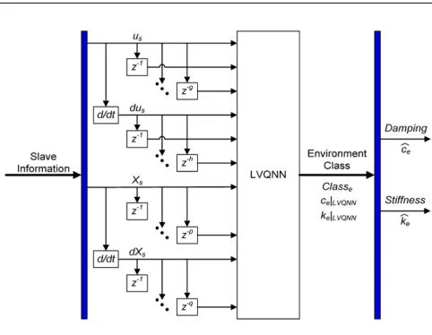
A LVQNN is employed to construct the NNEC in order to detect the environment characteristics in an online manner. For a LVQNN design, it is important to determine the input vector size and how many sequences of data use. Here, with the limited number of input information, the NNEC is built with: an input vector consisting of current and historical values of four signals: the slave driving command, {us(0), us(-1), …, us(-g)}, manipulator response, {Xs(0), Xs(-1), …, Xs(-p)}, and their derivatives, {du_s(0), du_s(-1), …, du_s(-n)} and {dX_s(0), dX_s(-1), …, dX_s(-q)}, respectively; an output vector containing the estimated values of the damping and stiffness, and , representing the environment class eth (classe). Configuration of the proposed classifier is described in Fig. 6. Due to uncertainties of the working environment, it is necessary to derive an algorithm to smoothly shift between different environment classes. Thus, a so-called smooth switching algorithm is proposed to determine the current environment based on the current class output from the LVQNN and the last detected class as

(4)

where λ is called forgetting factor.

Additionally, to avoid influences of noises on the NNEC performance, the forgetting factor is online tuned according to the changing speed of the classifier outputs, vY, which is defined by the number of sampling periods when the LVQNN outputs change continuously. The procedure to tune this factor can be expressed as:

Step 1: set initial value for the forgetting factor, λ = 0.5; define a small positive thresholds, 0 < γ₁ < γ₂, for vY.

Step 2: for each working step, check v_Y and update λ by comparing vY with its thresholds using the following rule:

+ If: (vY < γ2), Then: λ(t+ 1) =λ(t+ 1) / 2 and reset vY = 0; + Else If: (vY≥ γ1) & (vY(t) ≤ γ2), Then: λ(t+ 1) =λ(t+ 1)×2 and

reset vY = 0;

+ Otherwise, λ(t+ 1) = λ(t).

3.3 Fuzzy-based force feedback tuner

Although the environment characteristics are estimated using the NNEC, it is difficult to determine properly the FFG which is normally based on experience or prior knowledge about teleoperation systems. In decision making, many research works have shown that fuzzy logic which can take place of a skilled human operator is a feasible tool.20 Thus, in this research, the fuzzy-based feedback gain tuner and fuzzy cognitive map-based decision tool are proposed to compute the FFG.

3.3.1 Fuzzy feedback gain tuner

The FFGT is designed with two inputs, denoted as ke*, ce*, and single n_j D X W( , ₁( )j) (X i( )–W₁( )j i, )2

i=1 m

∑

= = j=1, ,…S₁

Y k( )=o₂( )k =k_W( )k n₂( )k

k_W( )k W₂( )k j, o₁( )j,

j=1 S₁

∑

= k=1, ,…n, (n S≡ ₂)

IF: X is classified correctly:

W₁t+1( )j =W₁t( )j +μ(X W– ₁t( )j ) Else: (X is classified inforrectly)

W₁t+1( )j =W₁t( )j –μ(X W– ₁t( )j) ⎩

⎪ ⎪ ⎨ ⎪ ⎪ ⎧

, j=1, ,…S₁

cˆ_e kˆ_e

cˆ

e( )t λ cˆ_{e class}

e(t–1)

× +(1–λ) cˆ

e LVQNN t( ) ×

=

kˆ_e( )t λ kˆ_{e class} e(t–1)

× +(1–λ)×kˆ_{e LVQNN t( )} =

⎩ ⎪ ⎨ ⎪ ⎧

Fig. 6 Configuration of the NNEC

output, k_f. The inputs are normalized values of the NNEC outputs:

(5)

where: gkand gc are the scaling factors.

The FFGT inspects the incoming system states, and transforms them into linguistic variables. Here, the linguistic variables of the stiffness and damping inputs are described in terms of ‘Low’, ‘Medium’, and ‘High’. Meanwhile, the gain output is described as ‘VS’ (Very Small), ‘S’ (Small), ‘M’ (Medium), ‘L’ (Large), ‘VL’ (Very Large). Triangle membership functions (MFs) are selected to represent these variables. These MFs are distributed over the FFGT input/output ranges as shown in Fig. 7. Next, the rule base is utilized to interpret expert knowledge in a useful way. It contains a set of conditional sentences in the form of (6). Subsequently, the rule table for this FGT is established in Table 2.

(6)

where Ai, Bj and Cij are the fuzzy subsets of the variables ke*, ce* and kf. The fuzzy inference is performed using the MAX-MIN operator. Let be MF of a subset of the output which is the result of rule R_ij. Then, it can be obtained by

(7)

Successively, the results of the nine rules are compared together to infer the final output MF μ_R(k_f) using the MAX operator:

(8)

The fuzzy decoder is finally used to produce the FFG gain, kf:

(9)

where and are in turn the maximum and minimum values of the FFG; Defuzzify (●) is the defuzzifier function which performs defuzzification by using the center average method.

3.3.2 Fuzzy cognitive map-based decision tool

Fuzzy cognitive maps (FCMs) are able to deal with processes like decision making that is based on human reasoning process21 and therefore, have been successfully used for many applications, ranging from medical fields, agricultural applications and environmental areas to energy problems.21-23 In this research, a FCM-based decision tool is developed to refine the FFG when considering the impacts of the estimated contact force, Fe, joystick moving speed change, , and upper limit of the gain k_f. This decision tool is built with a number of FFG decisive factors and knowledge of experts, along with the proper

selection of fuzzification and defuzzification functions.

3.3.3 Fuzzy cognitive map

An FCM designed for a system is graphically represented by a frame of nodes and connection edges. The nodes (or concepts) stand for different behaviours of the system. Each node can be an input/output variable, a state, or an event of the system. In addition, these nodes also interact with each other and therefore, are capable of representing the system dynamics. The interactions between nodes are modelled by connection edges of which the directions and weights indicate the directions and degrees of the causal relationships, respectively.

Each node can be denoted as C_i with i = 1, …, N (N is the number of FCM nodes) and characterized by a specific value, xi, which is fuzzified from the real system behaviour value into the closed universe [0, 1]. Between each two nodes, ith and jth, there are three possible relationships which are known as positive, negative or neutral causality and can be expressed by weight factors, w_ij, which are interpreted using linguistic variables in a normalized range [-1, 1]. A weight set of a generic FCM therefore can be defined as

(10)

The value, xi, of node Ci at step (k+1)th can be computed based on the influence of the other interconnected nodes, Cj, on node Ci, as

(11)

where f is an activation function which is selected based on different applications.

[ ]

[ ]

* ˆ_, * _ˆ, * _{0,1 ,} * _0,1

e k e e c e e e

k =g ×k c =g ×c k ∈ c ∈

(

)

* *

RuleRij: ifk is Ae iand isc Be jthenk isCf ij, i j, =1, 2,3

μR_ij( )kf

( )

(

( ) ( )

( )

)

µ = µ µ µ

( )

(

( )

( )

( )

)

R kf R kf R kf R kf

µ = µ µ µ

( )

(

)

(

)

f R f f f

k =Defuzzify µ k × k −k +k

k_f k_f

X··m

[ ]

1,1 1,

,1 ,

; 1,1 ; , 1,..., N

ij

N N N

w w

W w i j N

w w

⎡ ⎤

⎢ ⎥

=_{⎢ ⎥} ∈ − =

⎢ ⎥

⎣ ⎦

L

M O M

L

1

1, N

k k k

i i j ji

j j i

x+ f x x w

= ≠

⎛ ⎞

= ⎜ + ⎟

⎝

∑

Table 2 Rule table design for the FFGT

FFG (kf) Normalized estimated stiffness ke* Low Medium High

Normalized estimate damping ce*

Low VL L M

Medium L M S

High M S VS

Fig. 8 Fuzzy cognitive map design for FFG decisive factors

3.3.4 FCMD tool design

Four nodes (C1 to C4) standing for the estimated contact force, the

joystick moving speed change, variations of the feedback gain and its upper limit (denoted in turn as _δkf, and ) are selected to design the FCMD tool. The values of these nodes, x₁ to x₄, are then in turn the normalized values of , , δkf, and .

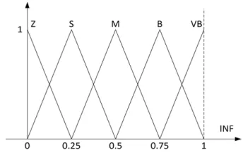
First, the influence between the FCMD nodes are analyzed. Based on the design experience, the interrelation between these nodes are defined as in Fig. 8. Due to the symmetric design of weight factors, their amplitude tagged as ‘INF’ can be represented by linguistic variables while their signs are defined by the direction of the connection edges in Fig. 8. These connection edge directions are determined based on experience of the experts. Here, five triangle membership functions tagged as ‘Z’, ‘S’, ‘M’, ‘B’, and ‘VB’, which in turn stand for zero, small, medium, big, and very big, are uniformly distributed within the closed universe [0, 1] to describe the influence (see Fig. 9). For decision making, it is realized that sigmoid and tansig (hyperbolic tangent sigmoid) functions are the two feasible choices.24 In this case, the tansig function is selected as the FCMD activation function:

(12)

where λ is the steepness parameter and selected as 2.

Therefore, the feedback gain and its upper limit can be updated for each working step as

(13)

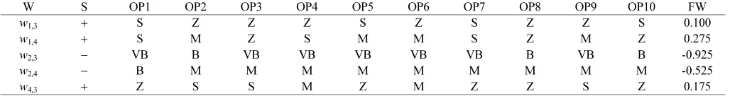
Second, the definition of the FCMD weights is carried out through an analysis on a series of teleoperation tests which were performed by 10 different operators. During the tests, each operator adjusted manually the FFG in order to make a proper force feedback sense to his/her hand. Through the tests, a survey on the impacts between the decisive factors has been performed by the operators. Based on their evaluation sheets (as summarized in columns OP1 to OP10 of Table 3), the final decision on FCMD weights is made by the defuzzification which is based on the centre average algorithm. By combining with the signs of the FCMD weights based on (column WS of Table 3), their final values are derived as the last column in Table 3.

4. Local Robust Adaptive Controller

The local robust adaptive controller (LRAC) is designed for the implementation to the slave manipulator and the master FFM (as the

SRAC and MRAC) to ensure their accurate position and pressure tracking performances, respectively. This LRAC is designed as a proportional-integral-derivative (PID) -based neural network in which the network is structured based on the well-known PID algorithm and their weights are trained online under a Lyapunov stability constrain. The LRAC is generally built for a system with one control input, u, and n outputs (in this case, u is the driving command for the control valve 1 or 2; n = 1, means one output which is the piston displacement or the reflected pressure). The network composes of three layers: an input layer as a control error sequence, a hidden layer with three nodes, tagged as P, I, and D, and an output layer, which is the system control input. The error sequence is defined as , where = ; and are in turn the desired system response and the actual response. Define { , , } is a weight vector of the hidden nodes with respect to input ith, and { , , } is the weight vector of the output layer. By applying the PID algorithm, the weights of the output layer are selected as unit while the output from each hidden node is derived as

(14)

Then, the output from the network is obtained using a linear function:

(15)

To ensure the adaptability of the LRAC, the back-propagation and gradient descent method is employed to tune the network weights. Additionally, a Lyapunov stability condition is integrated with the learning algorithm to guarantee the system robustness.

Learning algorithm: define a prediction error function as

(16)

The hidden weights can be online tuned for each step, (k+1)th, as:

(17)

where , , are the learning rates within [0,1]; the other factors in Eq. (17) are derived using partial derivative of the error function Eq. (16) with respect to each decisive parameter and chain rule method.25

Theorem 1: by selecting properly the learning rates in Eq. (17) for step (k+1)th to satisfy Eq. (18), then the stability

δkf

Fˆ_e X··m δkf

f a( ) 2 1+e–λa --- 1– =

(

)

(

)

1 0 0 ₁

1 1 ₁ 1

f f f

f f

k _k

f f

k k k

f FFGT

k k k k k

k k k

δ δ + ₊ + + + ⎧ _{= + −} ⎪ ⎨ ⎪ = + ⎩

eNN_k ={e_k1, ,…en_k–1} e_ki y_kdesired i, – y_kactual i, y_kdesired i, y_kactual i,

w_kPi w_kIi w_kDi w_kP w_kI w_kD

1 1 1 1 1 1 1 1 1 1 1

Node P : ;

Node I : ;

Node D :

n

P Pi i

k i k k

n

I I Ii i

k k i k k

n n

D Di i Di i

k i k k i k k

O w e

O O w e

O w e w e

− = − − = − − − − = = = = + = +

∑

∑

∑

∑

( )

k k k k k k

u = f O ≡O =O +O +O

(

)

( )

1 _{, ,} 1

1 1

, ,

0.5 n desired i 0.5 n

NN actual i i

k _i k k _i k

desired i

i actual i k k k

E y y e

e y y

− − = = = − = ≡ −

∑

∑

Pi Pi Pi Pi Pi NN Pi

k k k k k k k

Ii Ii Ii Ii Ii NN Ii

k k k k k k k

Di Di Di Di Di NN Di

k k k k k k k

w w w w E w

w w w w E w

w w w w E w

η η η + + +

⎧ = + Δ = − ∂ ∂

⎪

= + Δ = − ∂ ∂

⎨

⎪ _{= + Δ = − ∂ ∂}

⎩ ηk Pi _η k Ii _η k Di ηk Pi _η k Ii _η k Di

≡ ≡ =ηk

Table 3 Weight evaluation performed by different operators

W S OP1 OP2 OP3 OP4 OP5 OP6 OP7 OP8 OP9 OP10 FW

w1,3 + S Z Z Z S Z S Z Z S 0.100

w1,4 + S M Z S M M S Z M Z 0.275

w2,3 − VB B VB VB VB VB VB B VB B -0.925

w2,4 − B M M M M M M M M M -0.525

w4,3 + Z S S M Z M Z Z S Z 0.175

of the LRAC is guaranteed.

(18)

where .

Proof: by defining a Lyapunov function as Eq. (19), the change of this function is derived as Eq. (20)

(19)

(20)

From the controller structure, one has:

(21)

here, the terms , , and are obtained from Eq. (17). By using partial derivative and selecting , Eq. (21) becomes:

(22)

From Eqs. (22), (20) is rewritten as

(23)

The tracking performance is guaranteed to be stable only if

≤ 0, . It is clear that except η_k, the other factors in Eq. (23) can be determined online based on the prediction error and the chain rule method.25 Hence for each working step, it is easy to select a proper value of η_k to make Eq. (18) satisfy. Therefore, the proof is completed.

5. Experimental Results and Discussions

5.1 NNEC training and validation 5.1.1 Data acquisition

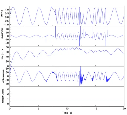
In order to utilize the NNEC supporting the SFFJC design, it is necessary to acquire data of the slave manipulator of the teleoperation test rig (see Fig. 3(d)) to characterize the environments as well as to train the NNEC. Open loop teleoperation experiments in which the input was the manipulator open loop driving command and the output was the manipulator displacement were performed on the test rig without activating the FFM and FSSC. Furthermore, to identify offline the environment characteristics, the pressure sensor attached to the salve cylinder was only employed for these tests to compute the interaction force between the slave and environment (Fig. 3(d)).

For each test, a trajectory was randomly given to the slave manipulator by the PC and the sampling period was set to 0.01 s. Besides the test in the free load condition (without attaching a spring), three among the five spring types in Table 1, type 1, 3 and 5, were selected to generate the three different environment classes for the

other three tests. The remained spring, types 2 and 4, were kept for the SFFJC validation to show the capability of this approach. Subsequently, the four sets of the slave input-output training data were observed. Fig. 10 displays a sample of open loop test result with respect to the spring type 1.

5.1.2 Environment characterization

Next, the acquired data sets were used to characterize the corresponding environments. In this case, the recursive least square method (RLSM) was applied to identify the stiffness of the selected spring types (assumed to be unknown as the practical applications). The environment model could be represented as

(24)

where Fe0 was the nonzero amount of the loading force at the initial

position of the slave.

For each environment, by replacing P sets of input-output data points of the slave positions and loading forces observed at P sampling intervals into Eq. (24), a matrix relation was obtained:

(25)

where: X was an unknown column vector including the parameters, k and F0; B was the loading force vector; A was a Px2 matrix of which

each row was described as (the superscript p denotes pth sample of the slave position).

Let define row ith of matrix A in Eq. (25) as a_i and element ith of vector B as bi, by using the RLSM,26X could be calculated iterativelyas:

(26)

where T_i was the covariance matrix.

The initial conditions to launch the algorithm Eq. (26) were X0 =0

(

)

1 ₂

1 0.5 0

n _i

k k k k

i e F Fη

−

= + ≤

∑

1

j NN j NN j NN

n

k k k k k k

k Pi Pj Ii Ij Di Dj

j k k k k k k

e E e E e E

F

w w w w w w

− = ⎛ ∂ ∂ ∂ ⎞ = − ⎜ _∂ + _∂ + _∂ ⎟ ⎝ ⎠

∑

(

)

( )

1 _{, ,} 1

1 1

0.5 n desired i 0.5 n

NN actual i i

k _i k k _i k

V − y y − e

= = =

∑

∑

( ) ( )

(

)

( )

(

)

(

)

1 1 1

2 1 1 1 0.5 0.5 , n

NN i i

k i k k

n _{i i i i i i}

k k k k k k

i

V e e

e e e e e e

−

+ = +

−

+ =

Δ = −

= Δ + Δ = + Δ

∑

∑

1

1

i i i

n

i k Pj k Ij k Dj

k Pj k Ij k Dj k

j k k k

e e e

e w w w

w w w

−

=

⎛ ∂ ∂ ∂ ⎞

Δ = ⎜_∂ Δ +_∂ Δ +_∂ Δ ⎟

⎝ ⎠

∑

≡ ≡ =ηk

i k k k

e η F

Δ =

(

)

1 2

1 ₁ 0.5

n

NN i

k _i k k k k

V+ ₌− e F Fη

Δ =

∑

V_kNN₊₁ Δ k

∀

F_e=k_eX_s+F_e0

AX=B

X_sp 1

[ ]

1 1 1 1 1

1 1 1

1 1

( )

, 0,1,..., 1 1

T

i i i i i i i

T i i i i

i i T

i i i

X X T a b a X

T a a T

T T i P

a T a

+ + + + + + + + + + = + − = − = − +

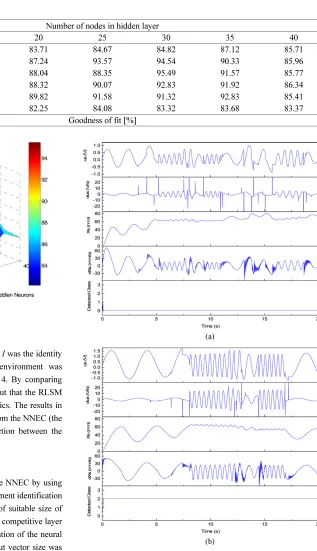
and T0 = γI, where γ was a positive large number and I was the identity

matrix of dimension 2 × 2. Subsequently, the environment was characterized for each test case as shown in Table 4. By comparing with the actual spring stiffness, the results pointed out that the RLSM could identify precisely the environment characteristics. The results in Table 4 were then used to combine with the output from the NNEC (the detected environment class) to estimate the interaction between the slave and environment.

5.1.3 NNEC optimization

Next, the training progress was carried out for the NNEC by using the data sets obtained in Section 5.1.1 and the environment identification results derived in Section 5.1.2. The determination of suitable size of the input vector and number of hidden neurons in the competitive layer is one of the essential issues in practical implementation of the neural network-based classifier (Section 3.2). Here, the input vector size was defined based on the numbers of time-based data points of the available signals, us and Xs. The training was performed with the different

settings of the input layer and hidden layer, in which the number of inputs was changed from 20 to 40 and the number of hidden neurons was varied from 10 to 40. The correlation between the network output and target output (the environment class) was used to describe the

training success. The training result (goodness of fit [%]) of the NNEC was then analyzed in Table 5 and Fig. 11.

Table 4 Environment characterization results

Environment class (Spring type) Actual Stiffness N/m RLSM-based Stiffness N/m Identification Accuracy [%]

Class 0 (Free Load) 0 -

-Class 1 (Spring type 1) 500 509.649 98.070

Class 2 (Spring type 3) 1500 1531.047 97.930

Class 3 (Spring type 5) 2500 2550.731 97.978

Table 5 Learning success rate of NNEC [%]

Number of inputs

Number of nodes in hidden layer

10 15 20 25 30 35 40

20 84.43 84.66 83.71 84.67 84.82 87.12 85.71

24 86.44 84.91 87.24 93.57 94.54 90.33 85.96

28 86.25 83.82 88.04 88.35 95.49 91.57 85.77

32 85.44 84.90 88.32 90.07 92.83 91.92 86.34

36 84.15 85.88 89.82 91.58 91.32 92.83 85.41

40 84.16 85.40 82.25 84.08 83.32 83.68 83.37

Goodness of fit [%]

Fig. 11 Goodness of fit - 3D map

From these results, it can be found that the most suitable NNEC structure was realized with 28 nodes in the input vector and 30 nodes in the competitive layer. The learning success rate in this case was highest with 95.49 [%]. The result implies that the designed NNEC could estimate well the working environment at the slave site.

5.1.4 NNEC validation

To validate the applicability of the optimized NNEC, real-time open loop experiments on the test rig were performed. During these experiments, the cylinder was randomly driven by the PC and, the NNEC was employed to detect the environment conditions. Here, the environment was set to the class 0 (free load) and class 2 (using the spring type 3). Subsequently, the NNEC detection performances were obtained as plotted in Fig. 12(a) and 12(b). These results show that the classifier could detect the loading conditions and the outputs reached stably and accurately to the true classes in a short time. This confirm convincingly that the proposed classifier could identify online correctly the environment class. By combining with the environment characterization results (as presented in Section 5.1.2), it is therefore capable of producing precisely the environment characteristics which take an important task in setting the desired reflection force.

5.2 LRAC Verification

Experiments with the FFM pressure tracking control and cylinder position tracking control were done separately to investigate the capability of the local controllers, MRAC and SRAC, respectively. For each control objective, a comparative study of the designed controller and a conventional PID controller was carried out. Due to the fixed gain use, the PID control gains were manually tuned for each given trajectory by using the following steps:

Step 1: the control objective was approximated by a transfer function derived from its data using system identification toolbox of Matlab27;

Step 2: for each tracking trajectory, the PID gains were tuned for the derived system transfer function using PID tuner of Matlab/Simulink; Step 3: the PID gains obtained from Step 2 were refined through control tests with the real system.

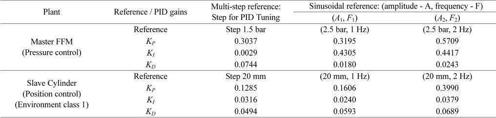
Sinusoidal and multi-step signals were used to generate tracking profiles for the tests. Based on the test rig specifications, the parameters of these profiles were properly determined. Consequently, the PID gains were derived for each test case as shown in Table 6. It is note that in Table 6 with the position tracking, the PID gains were tuned for the case that the environment was the class 1 (using the spring type 1).

5.2.1 Rotary actuator pressure tracking control

First, experiments were carried out with the rotary actuator pressure control using the two controllers, PID and MRAC. The comparison results with respect to the multi-step and sinusoidal references were obtained and in turn plotted in Figs. 13 and 14. When dealing with the multi-step reference, the performances of both the controllers were quite similar with acceptable control error. However, by using the PID controller, of which the gains were tuned for the small jumping step (1.5 bar), the responses of the actuator to the larger jumping steps were slower than those of using the MRAC. The differences between these control performances were bigger in case of sinusoidal tracking. Although the tuned PID controller could drive the system to follow the desired goal quickly with acceptable error, this steady state error (SSE) was larger than that of the MRAC controller (±0.2 bar compared to

±0.05 bar in case of the 1 Hz reference). The PID performance was continuously degraded at the higher frequency, 2 Hz with larger SSE. Meanwhile, the MRAC could always ensure the fast response and small SSE in both the test cases (less than ±0.075 bar, equivalent to

±3% of the sinusoidal trajectory amplitude). The reason was that the MRAC was the advanced combination between the adaptive neural network and robust learning technique to compensate the system nonlinearities and uncertainties and therefore, minimize the control error.

5.2.2 Cylinder position tracking control

Next, experiments were carried out with the cylinder position control Table 6 Setting parameters for test profiles and PID controllers

Plant Reference / PID gains Multi-step reference: Step for PID Tuning

Sinusoidal reference: (amplitude - A, frequency - F) (A1, F1) (A2, F2)

Master FFM (Pressure control)

Reference Step 1.5 bar (2.5 bar, 1 Hz) (2.5 bar, 2 Hz)

KP 0.3037 0.3195 0.5709

KI 0.0029 0.4305 0.4417

KD 0.0744 0.0180 0.0243

Slave Cylinder (Position control) (Environment class 1)

Reference Step 20 mm (20 mm, 1 Hz) (20 mm, 2 Hz)

KP 0.1285 0.1606 0.3990

KI 0.0316 0.0240 0.0379

KD 0.0494 0.0593 0.0689

using the two controllers, SRAC and PID (Table 6). Similar to the pressure tracking control tests, the two controllers were in turn applied to drive the cylinder to follow the trajectories defined in Table 6 in different load conditions. Herein, the environment classes 1 and 3 in Table 4 were employed for the tracking control tests. The comparison results were obtained as plotted in Figs. 15 to 17. As denoted in Table 6, the PID control gains were derived for the system working in the environment class 1. Hence, when the environment class 1 was selected, the tracking results using the compared controllers were both acceptable as shown in Fig. 15. The PID controller, with the gains optimized manually for the working step 20 mm and environment class 1, could achieved the small SSE in the small working steps. This SSE was increased together with the rise of undershoots when the system faced with the large step changes. Similarly, the control performance was degraded when the external environment was varied from the class 1 to class 3. This phenomenon is clearly shown through the PID control results with respect to the sinusoidal references.

Without changing the environment condition, compared to the condition to derive the PID gains, the controller could drive the system to reach the goals with small SSE (within ±1.2 mm, corresponding to 6% of the reference amplitude) in both the two working frequencies (Figs. 16 and 17). Once the environment was changed, the performance was significantly deteriorated with large SEE (around ±3.8 mm, corresponding to ±19% of the reference amplitude). On the contrary, Fig. 14 Pressure tracking results: (a) Sine 1 Hz, (b) Sine 2 Hz

Fig. 15 Position tracking results: multi-step trajectory (a) Environment class 1; (b) Environment class 3

by using the SRAC with the same advanced functionalities as the MRAC, the best tracking results with small overshoot, fast rising time and small SSE were achieved in both the cases (Figs. 15 to 17). The tracking accuracy using the SRAC was always guaranteed to be less than ±0.5 mm (±2.5% of the trajectories’ amplitudes).

From the comparative studies with both the local controllers, SRAC and MRAC, it can be concluded that these designed controllers are powerful for the teleoperation control application.

5.3 SFFJC verification

In this section, the full control system, SFFJC, has been applied to the test rig (Fig. 3) in order to evaluate its applicability to teleoperation applications. A series of experiments on the testing system was conducted under the three different environment classes. Here, to investigate the adaptability of the SFFJC, the spring types 1, 2, and 4 from Table 1 were chosen to represent the environment. Additionally, in order to create challenges for the control system in detecting the environment changes as well as keeping the stability of the FFM rotary actuator and slave manipulator, these springs were installed so that they were initially in the free lengths (by adjusting the lock position of the slider in Fig. 3(d)). The springs were only compressed when the cylinder rod moves forward a pre-defined distance. In this study, this distance was set to 7 mm. The joystick commands were randomly given by the operator to drive the slave manipulator. Based on an analysis of the operator-joystick and slave dynamics and using the trial-and-error method, the

transformed factor was properly assigned by 1/4.5, which means a 4.5 N reflected force was equivalent with a 1 bar reflected pressure.

The closed loop teleoperation experiments were then performed and the results are plotted in Figs. 18 to 20. From these figures, it can be seen that the proposed SFFJC behaved well with high accuracy. This comes as no surprise because the SFFJC possesses the three advanced modules: FSSC, MRAC and SRAC. With the FSSC implementation, the environment characteristics in either free-load or load condition could be estimated accurately by the NNEC. As shown in the third and second sub-plots from the bottom of Figs. 18-20, the environment classes were determined correctly as 1, 1.5 and 2.5 which were correspond with the actual spring selection, type 1, type 2 and type 4. Moreover, the NNEC could detect immediately the change of external environment, from free load (indicated by the free load region in the top sub-plots) to load and vice versa. Based on this estimation, the FFFT was capable of producing properly the desired reflected pressure by regulating smoothly the FFG in order to make the similar load feeling to the master site (see the first sub-plots from the bottom of Figs. 18-20). Next, the two local controllers took parts in executing precisely the tasks given to the slave manipulator and the master FFM (cylinder position control and rotary actuator pressure control). The control results, which are in turn depicted in the fourth and fifth sub-plots of Figs. 18-20 (from the bottom), proved remarkably the capability of these controllers. As a result, the proposed SFFJC could ensure the stable performance for the teleoperation system in which the slave Fig. 17 Position tracking results - Environment class 3: (a) Sine 1 Hz

performed accurately the desired task while the operator was able to realize truthfully the interaction between the slave manipulator and the environment.

6. Conclusions

This paper presents the simple, safe and cost-effective approach named sensorless force feedback joystick control for teleoperation applications, especially in construction sector. The main contributions of this study can be summarized as follows:

+ The force sensorless supervisory controller is designed as the combination of the neural network-based environment classifier and the fuzzy-based force feedback tuner. The NNEC is capable of detecting the environment characteristics at the slave site without requiring any sensor to estimate the interaction between the slave and environment. Meanwhile, the FFFT with the fuzzy-based cognitive map decision tool is capable of deriving appropriately the target reflecting pressure for the FFM based on the NNEC outputs.

+ The two robust adaptive controllers, SRAC and MRAC, are implemented to ensure the adaptability and stability of the position and pressure tracking of the closed loop slave and master systems.

+ By integrating both the advanced characteristics of the FSSC, SRAC and MRAC into the SFFJC, the acceptable teleoperation performance could be always achieved disregarding the system

nonlinearities and uncertainties. The experimental results then prove convincingly the effectiveness of the proposed control approach.

It should be noted that the focus of this paper is to develop the SFFJC approach over wired communication. Therefore, the presence of time delays over communication channels of a teleoperation system is not considered here. The delay problems and/or data packet losses normally existing in wireless or network-based control systems have been carefully addressed and separately resolved by the authors as presented in our recent publications.28-30 As an area of the future work, the development of a SFFJC-based teleoperation control system with imperfect communication using the results of our current studies is carrying out in order to widen its applicability. Another aspect of the future work is to investigate the capability of the proposed control approach when dealing with multi-DOF teleoperation systems.

ACKNOWLEDGEMENT

This work is supported by the “Next-generation construction machinery component specialization complex development program through the Ministry of Trade, Industry and Energy (MOTIE) and Korea Institute for Advancement of Technology (KIAT), and the Innovate UK through the Off-Highway Intelligent Power Management (OHIPM, Project Number: 49951-373148 in collaboration with the WMG Centre High Value Manufacturing (HVM), JCB and Pektron).

REFERENCES

1. Shams, S., Kim, D. S., Choi, Y. S., and Han, C. S., “A Novel 3-DOF Optical Force Sensor for Wearable Robotic Arm,” Int. J. Precis. Eng. Manuf., Vol. 12, No. 4, pp. 623-628, 2011.

2. Park, W.-I., Kwon, S., Lee, H.-D., and Kim, J., “Real-Time Thumb-Tip Force Predictions from Noninvasive Biosignals and Biomechanical Models,” Int. J. Precis. Eng. Manuf., Vol. 13, No. 9, pp. 1679-1688, 2012.

3. Jung, K., Chu, B., Park, S., and Hong, D., “An Implementation of a Teleoperation System for Robotic Beam Assembly in Construction,” Int. J. Precis. Eng. Manuf., Vol. 14, No. 3, pp. 351-358, 2013.

4. Je, H.-W., Baek, J.-Y., and Lee, M. C., “Current Based Compliance Control Method for Minimizing an Impact Force at Collision of Service Robot Arm,” Int. J. Precis. Eng. Manuf., Vol. 12, No. 2, pp. 251-258, 2011.

5. Islam, S., Liu, P. X., and El Saddik, A., “New Stability and Tracking Criteria for a Class of Bilateral Teleoperation Systems,” Information Sciences, Vol. 278, pp. 868-882, 2014.

6. De Gersem, G., “Kinaesthetic Feedback and Enhanced Sensitivity in Robotic Endoscopic Telesurgery,” Catholic University of Leuven, 2005.

7. Lee, J. K., Kim, K. H., and Kang, M. S., “An Analysis of Static Output Feedback Control for Tendon Driven Master-Slave Manipulator - Simulation Study,” Int. J. Precis. Eng. Manuf., Vol. 12, No. 2, pp. 243-250, 2011.

8. Ahn, K. K., “Development of Force Reflecting Joystick for Hydraulic Excavator,” JSME International Journal Series C Mechanical Systems, Machine Elements and Manufacturing, Vol. 47, No. 3, pp. 858-863, 2004.

9. Kuchenbecker, K. J. and Niemeyer, G., “Induced Master Motion in Force-Reflecting Teleoperation,” Journal of Dynamic Systems, Measurement, and Control, Vol. 128, No. 4, pp. 800-810, 2006.

10. Polushin, I. G., Liu, P. X., and Lung, C.-H., “Projection-Based Force Reflection Algorithm for Stable Bilateral Teleoperation Over Networks,” IEEE Transactions on Instrumentation and Measurement, Vol. 57, No. 9, pp. 1854-1865, 2008.

11. Polushin, I. G., Liu, X. P., and Lung, C.-H., “Stability of Bilateral Teleoperators with Generalized Projection-Based Force Reflection Algorithms,” Automatica, Vol. 48, No. 6, pp. 1005-1016, 2012.

12. Kim, D., Oh, K. W., Lee, C. S., and Hong, D., “Novel Design of Haptic Devices for Bilateral Teleoperated Excavators Using the Wave-Variable Method,” Int. J. Precis. Eng. Manuf., Vol. 14, No. 2, pp. 223-230, 2013.

13. Moreau, R., Pham, M. T., Tavakoli, M., Le, M. Q., and Redarce, T., “Sliding-Mode Bilateral Teleoperation Control Design for Master– Slave Pneumatic Servo Systems,” Control Engineering Practice, Vol. 20, No. 6, pp. 584-597, 2012.

14. Yang, T., Fu, Y., and Tavakoli, M., “Digital Versus Analog Control of Bilateral Teleoperation Systems: A Task Performance Comparison,” Control Engineering Practice, Vol. 38, pp. 46-56, 2015.

15. Kim, W. S., Hannaford, B., and Fejczy, A. K., “Force-Reflection and Shared Compliant Control in Operating Telemanipulators with Time Delay,” IEEE Transactions on Robotics and Automation, Vol. 8, No. 2, pp. 176-185, 1992.

16. Kotsiantis, S. B., “Supervised Machine Learning: A Review of Classification Techniques,” Informatica, Vol. 31, pp. 249-268, 2007.

17. Singh, J. and Nene, M. J., “A Survey on Machine Learning Techniques for Intrusion Detection Systems,” International Journal of Advanced Research in Computer and Communication Engineering, Vol. 2, No. 11, pp. 4349-4355, 2013.

18. Sharif, M. S., Abbod, M., Amira, A., and Zaidi, H., “Artificial Neural Network-Statistical Approach for PET Volume Analysis and Classification,” Advances in Fuzzy Systems, Vol. 2012, Article No. 5, 2012.

19. Schneider, P., Biehl, M., and Hammer, B., “Adaptive Relevance Matrices in Learning Vector Quantization,” Neural Computation, Vol. 21, No. 12, pp. 3532-3561, 2009.

20. Truong, D. Q. and Ahn, K. K., “Force Control for Hydraulic Load Simulator Using Self-Tuning Grey Predictor-Fuzzy PID,” Mechatronics, Vol. 19, No. 2, pp. 233-246, 2009.

21. Kyriakarakos, G., Patlitzianas, K., Damasiotis, M., and Papastefanakis, D., “A Fuzzy Cognitive Maps Decision Support System for Renewables Local Planning,” Renewable and Sustainable Energy Reviews, Vol. 39, pp. 209-222, 2014.

22. Stylios, C. D., Georgopoulos, V. C., Malandraki, G. A., and Chouliara, S., “Fuzzy Cognitive Map Architectures for Medical Decision Support Systems,” Applied Soft Computing, Vol. 8, No. 3, pp. 1243-1251, 2008.

23. Yaman, D. and Polat, S., “A Fuzzy Cognitive Map Approach for Effect-Based Operations: An Illustrative Case,” Information Sciences, Vol. 179, No. 4, pp. 382-403, 2009.

24. Bueno, S. and Salmeron, J. L., “Benchmarking Main Activation Functions in Fuzzy Cognitive Maps,” Expert Systems with Applications, Vol. 36, No. 3, pp. 5221-5229, 2009.

25. Truong, D. Q. and Ahn, K. K., “Nonlinear Black-Box Models and Force-Sensorless Damping Control for Damping Systems Using Magneto-Rheological Fluid Dampers,” Sensors and Actuators A: Physical, Vol. 167, No. 2, pp. 556-573, 2011.

26. Åström, K. J. and Wittenmark, B., “Computer-Controlled Systems: Theory and Design,” Dover Publications, Inc., 3rd Ed., 2013.

27. Ahn, K. K. and Truong, D. Q., “Self-Tuning of Quantitative Feedback Theory for Force Control of an Electro-Hydraulic Test Machine,” Control Engineering Practice, Vol. 17, No. 11, pp. 1291-1306, 2009.

Time Delay Measurement and a Smart Adaptive Unequal Interval Grey Predictor for Real-Time Nonlinear Control Systems,” IEEE Transactions on Industrial Electronics, Vol. 60, No. 10, pp. 4574-4589, 2013.

29. Truong, D. Q. and Ahn, K. K., “Robust Variable Sampling Period Control for Networked Control Systems,” IEEE Transactions on Industrial Electronics, Vol. 62, No. 9, pp. 5630-5643, 2015.