Private release of graph statistics using ladder functions

(1)

http://wrap.warwick.ac.uk

Original citation:

Zhang, Jun, Cormode, Graham, 1977-, Procopiuc, Cecilia M., Srivastava, Divesh and

Xiao, Xiaokui (2015) Private release of graph statistics using ladder functions. In: ACM

SIGMOD 2015, Melbourne, Australia, 1-4 Jun 2015. Published in: SIGMOD '15

Proceedings of the 2015 ACM SIGMOD International Conference on Management of

Data pp. 731-745.

Permanent WRAP url:

http://wrap.warwick.ac.uk/67368

Copyright and reuse:

The Warwick Research Archive Portal (WRAP) makes this work by researchers of the

University of Warwick available open access under the following conditions. Copyright ©

and all moral rights to the version of the paper presented here belong to the individual

author(s) and/or other copyright owners. To the extent reasonable and practicable the

material made available in WRAP has been checked for eligibility before being made

available.

Copies of full items can be used for personal research or study, educational, or not-for

profit purposes without prior permission or charge. Provided that the authors, title and

full bibliographic details are credited, a hyperlink and/or URL is given for the original

metadata page and the content is not changed in any way.

Publisher’s statement:

"© ACM, 2015. This is the author's version of the work. It is posted here by permission of

ACM for your personal use. Not for redistribution. The definitive version was published in

SIGMOD '15 Proceedings of the 2015 ACM SIGMOD International Conference on

Management of Data pp. 731-745 (2015)

http://doi.acm.org/10.1145/2723372.2737785

"

A note on versions:

The version presented here may differ from the published version or, version of record, if

you wish to cite this item you are advised to consult the publisher’s version. Please see

the ‘permanent WRAP url’ above for details on accessing the published version and note

that access may require a subscription.

(2)

Private Release of Graph Statistics using Ladder Functions

Jun Zhang

1

_{Graham Cormode}

2

_{Cecilia M. Procopiuc}

3∗

_{Divesh Srivastava}

4

_{Xiaokui Xiao}

1

1_{Nanyang Technological University} 2_{University of Warwick}

{jzhang027, xkxiao}@ntu.edu.sg

[email protected]

3_{Google Inc.} 4_{AT&T Labs – Research}

ABSTRACT

Protecting the privacy of individuals in graph structured data while making accurate versions of the data available is one of the most challenging problems in data privacy. Most efforts to date to per-form this data release end up mired in complexity, overwhelm the signal with noise, and are not effective for use in practice. In this paper, we introduce a new method which guarantees differential privacy. It specifies a probability distribution over possible outputs that is carefully defined to maximize the utility for the given input, while still providing the required privacy level. The distribution is designed to form a ‘ladder’, so that each output achieves the highest ‘rung’ (maximum probability) compared to less preferable outputs. We show how our ladder framework can be applied to problems of counting the number of occurrences of subgraphs, a vital objective in graph analysis, and give algorithms whose cost is comparable to that of computing the count exactly. Our experimental study confirms that our method outperforms existing methods for count-ing triangles and stars in terms of accuracy, and provides solutions for some problems for which no effective method was previously known. The results of our algorithms can be used to estimate the parameters of suitable graph models, allowing synthetic graphs to be sampled.

Categories and Subject Descriptors

H.2.7 [Database Administration]: Security, integrity & protection

Keywords

Differential privacy; subgraph counting; local sensitivity

1. INTRODUCTION

A large amount of private data can be well-represented by graphs. Social network activities, communication patterns, dis-ease transmission, and movie preferences have all been encoded as graphs, and studied using the tools of graph theory. Given the pri-vate nature of the information stored in graphs, and the increasing

∗_{Author worked on this result while she was at AT&T Labs.}

Permission to make digital or hard copies of all or part of this work for personal or classroom use is granted without fee provided that copies are not made or distributed for profit or commercial advantage and that copies bear this notice and the full cita-tion on the first page. Copyrights for components of this work owned by others than ACM must be honored. Abstracting with credit is permitted. To copy otherwise, or re-publish, to post on servers or to redistribute to lists, requires prior specific permission and/or a fee. Request permissions from [email protected].

SIGMOD’15,May 31–June 4, 2015, Melbourne, Victoria, Australia. Copyrightc 2015 ACM 978-1-4503-2758-9/15/05 ...$15.00.

pressure to allow controlled release of private data, there has been much interest in ways to do so with some guarantee of anonymity.

The current locus of privacy work is around differential privacy. The model is popular, since it offers both provable properties on the results and practical algorithms to provide them. It is a statis-tical model of privacy which ensures that the output of the process undergoes sufficient perturbation to mask the presence or absence of any individual in the input. This model is very effective for re-leasing data in the form of histograms or counts, since the magni-tude of the statistical noise is often dominated by random variation in the data. Applying this model to graph data has proven much more fraught. The main technical roadblock is that direct appli-cation of standard methods seems to require such a large scale of random modification of the graph input as to completely lose all its properties. Concretely, any method which tries to directly output a modified version of the input graph under differential privacy is indistinguishable from random noise.

Instead, progress has been made by focusing on releasing prop-erties of the input graph under differential privacy, rather than the graph itself. For example, it is straightforward to release the num-ber of nodes and edges with this guarantee, by appealing to stan-dard techniques. It is valuable to find statistical properties of the graph, since there are many random graph models which take these as parameters (e.g., Kronecker graph models [26] and Exponen-tial Random Graph Models [17]), and allow us to sample graphs from this family, which should have similar properties to the input graph. The properties of the graph are also important in their own right, determining, for instance, measures of how much clustering there is in the graph, and other characteristics of group behavior. See the discussion in [17], and references therein.

The problem then becomes one of providing effective ways to release statistics on the input graph privately. The most impor-tant statistics aresubgraph counts: the number of occurrences of particular small subgraphs within the input graph. This remains a challenging problem, since standard differential privacy techniques still add a large amount of noise to the result. Take as a canonical problem the question of counting the number of triangles within a graph. The presence or absence of one relationship (represented by an edge) in the graph can contribute to a large number of potential triangles, and so the noise added to the count has to be scaled up by this amount. There have been numerous prior attempts to privately release statistics on graphs via more complex methods, but these still suffer from high noise, and high running time.

(3)

mecha-triangle(4) 3-star(3?) 4-clique(4C) 2-triangle(24)

Figure 1: Examples of subgraphs

nism and a carefully tuned quality function. We combine these in a new way to define a class of “ladder functions”, which provide the optimal sampling distribution for outputs. When applied to sub-graph counting queries, the results are efficient to compute, and improve substantially over prior work on these problems, where applicable.

1.1 Our Contributions

We show how to answer subgraph counting queries in a differ-entially private manner [7]. Given a subgraphH, e.g., a triangle, we aim to release the number of isomorphic copies ofHin the sen-sitive graph, while protecting individual privacy in the meantime. We writefH(g)to denote the function that computes the number of

copies of subgraphHin graphg. We focus on a number of impor-tant classes ofH. The functionf4counts the number of triangles in the graph: this is the most heavily studied subgraph counting query, as the triangle is the smallest non-trivial subgraph of interest. Other important subgraph counting functions include:fk?, for countingk

-stars (one node of degreekconnected toknodes of degree 1); fk_C,

for countingk-cliques; and fk4for countingk-triangles (a pair of adjacent nodesi,jthat havekcommon neighbors). Figure 1 shows the smallest non-trivial example of each of these classes: note that the 3-clique and the 1-triangle are simply the standard triangle.

We draw up the following list of criteria that our desired solution for differentially private subgraph counting should satisfy: 1. The solution should achieve pure differential privacy;

2. It should be applicable to a wide range of queries, e.g., triangle counting,k-star counting,k-triangle counting andk-clique counting for a constantk;

3. Its time complexity should be no larger than that of computing the true query answer for the queries of interest;

4. It should have high accuracy on its output, bettering that of any previous applicable solution.

Outline of Ladder Framework Development.Our ladder frame-work achieves all the above criteria. It relies on the careful design of a probability distribution for outputting answers to count queries that tries to maximize the probability of outputting the true answer, or one that is near to it, and minimize the probability of outputting answers that are far from the true answer. The framework of differ-ential privacy places constraints on how these probabilities should behave: the probability of providing outputxfor input graph g

should be “close” (as determined by the parameterε) to that for input graphg0, ifgandg0are close (differ by one edge). Rather than go right back to first principles to design these probability dis-tributions, we make use of the exponential mechanism [25], since this approach is general: any differentially private mechanism can be expressed as an exponential mechanism.

Instantiating the exponential mechanism still takes some care-ful design. We arrive at the design of a symmetric “ladder func-tion” specific to the input graphg, so-called because it is formed from a series of rungs. The first rung groups together a num-ber of outputs that are close to the true answer to fH(g) (i.e.

fH(g)±1,fH(g)±2. . .). The second rung groups together outputs

that are a little further away, and so on (see Figure 3). The height of each rung determines the probability of outputting the

correspond-ing values, while the width is the number of output values sharcorrespond-ing the same height. Ideally, we would make each rung as narrow as possible, to maximize the dropoff in probabilities away from fH.

However, to guarantee differential privacy, we need to make the rungs wide enough so that theith rung of the ladder forgoverlaps with thei−1st,ith ori+1st rung of the ladder for all neighboring

g0(in the language of the exponential mechanism, we seek bounded ‘sensitivity’ of the derived quality function). We call this the “small leap property”.

It turns out that we can design such ladder functions which have rungs that are not too wide but which satisfy the small leap prop-erty. Moreover, these can be computed efficiently from the input graphgand used to perform the required output sampling. Our de-velopment of these objects takes multiple steps. First, we fill in the necessary details of differential privacy (Section 2). Then we show how the use of ladder functions can lead to a practical differentially private solution, if we assume the small leap property, and that the functions converge to a constant rung width (Section 3). We still have to show that we can create such functions, and this is the focus of Section 4, where we show that the concept of “local sensitivity at distancet” can be used to create a ladder function with the re-quired properties. This provides a general solution which satisfies privacy; however, some of the quantities required can be time con-suming to compute for certain subgraph counting queries. Hence, Section 5 considers how to instantiate our framework for specific queries, and provides alternate ladder functions for some queries to enable efficient computation. Our experimental evaluation of this approach, and comparison with previous works (where applicable) is detailed in Section 6.

1.2 Previous Work on Subgraph Counting

An obvious first attempt to differentially private subgraph count-ing is to apply the Laplace mechanism [11]. The Laplace mecha-nism answers a (numeric) query f by adding Laplace noise to the true answer, where the scale of noise is proportional to theglobal sensitivityof f. The global sensitivity is defined as the maximum possible change of query answer if one tuple is added to/deleted from an arbitrary database. This method fails since the global sen-sitivity of subgraph counting queries is very large, making the noise large enough to overwhelm the true answer. In the case of triangles, for example, adding or deleting an edge can affect a number of tri-angles proportional to the number of nodes, and hence the global sensitivity is very high.

Nissim et al. [29] and Karwa et al. [17] present an idea of uti-lizing a local version of global sensitivity, calledlocal sensitivity, to build the noise distribution. The local sensitivity is a function of the input database, which is equal to the maximum change of query answer if one tuple is added in/deleted from the input database. The local sensitivity can be dramatically smaller than its global counter-part, but cannot be used directly to guarantee privacy. Instead, an upper bound on local sensitivity calledsmooth sensitivityis com-puted as a part of the noise scale. In [17], the authors give algo-rithms for computing smooth sensitivity of f4and fk?. However,

their idea fails when the smooth sensitivity of a query is hard to compute, e.g., fk4. In recompense, they propose an approach tai-lored specifically forfk4, which only achieves a restricted version of differential privacy.

(4)

Table 1: Table of notation

Notation Description

f,g the graph query and its sensitive input

Gn the set of simple graphs withnnodes

d(g,g0) minimum edit distance between two graphs

GS global sensitivity off LS(g) local sensitivity off, giveng

LS(g,t) local sensitivity offat distancet, giveng q(g,k) quality of outputk, given inputg

∆q sensitivity of quality functionq

It(g) the ladder function

withO(L)variables whereLequals the number of subgraphsHin the input times the number of edges inH. So the time complexity is super-quadratic in the answer value, making this method infeasible even for an input graph of moderate size (see details in Section 6).

Finally, Hay et al. [15] give a differentially private algorithm for publishing degree sequence of a sensitive graph. Since the number ofk-stars is a function of the degree sequence, this approach implic-itly allowsk-star counting. It first utilizes the Laplace mechanism to generate a private version of the degree sequence, then applies a postprocessing step to enforce consistency of the sequence in order to reduce noise. Though better than the naive Laplace mechanism, it is reported to be less accurate than the solutions in [17] onk -star counting (see Section 6.3 of [17]). We note that this method was not designed fork-star counting; also it doesnotsupport other counting queries discussed in this paper.

2. PRELIMINARIES

In this section, we review the definition of differential privacy, two conventional mechanisms to achieve differential privacy, and some basic concepts of local sensitivity. The notational conven-tions of this paper are summarized in Table 1.

2.1 Differential Privacy

Letg∈Gnbe a sensitive simple graph withnnodes, and fbe the

subgraph counting query of interest. Differential privacy requires that, prior to f(g)’s release, it should be modified using a random-ized algorithmA, such that the output ofAdoes not reveal much information about any edge ing. The definition of differential pri-vacy that we adopt in the context of graphs is as follows:

DEFINITION2.1 (ε-DIFFERENTIALPRIVACY[11, 15]). A randomized algorithmAsatisfiesε-differential privacy, if for any two graphs g and g0that differ by at most one edge, and for any possible output O ofA, we have

Pr[A(g) =O]≤eε_·_Pr

A(g0) =O, (1)

wherePr[·]denotes the probability of an event.

In what follows, we say that two graphsg,g0which differ by at most one edge are neighboring, i.e., their minimum edit distance [4]

d(g,g0)≤1. While there are many approaches to achieving dif-ferential privacy, the best known and most-widely used two for this purpose are theLaplace mechanism[11] and theexponential mech-anism[25].

The Laplace mechanism releases the result of a function f that takes as input a dataset and outputs a vector of numeric values. Given f, the Laplace mechanism transforms finto a differentially private algorithm by adding i.i.d. noise (denoted asη) into each

output value off. The noiseηis sampled from aLaplace distribu-tionLap(λ)with the following pdf: Pr[η=x] =₂1

λe

−|x|/λ_{. Dwork}

et al. [11] show that the Laplace mechanism achievesε-differential privacy ifλ≥GSf/ε, whereGSf is theglobal sensitivityof f. In

our problem setting (i.e., f is a subgraph counting query),GSf is defined as follows:

DEFINITION2.2 (GLOBALSENSITIVITY[11]). Let f be a function that maps a graph into a real number. The global sen-sitivity of f is defined as

GSf= max

g,g0_|_d₍_g,g0₎_≤1

f(g)−f(g0)

, (2)

where g and g0are any two neighboring graphs.

Intuitively,GSfmeasures the maximum possible change inf’s out-put when we modify one arbitrary edge in f’s input.

For an analysis taskfwith a categorical output (e.g., a zipcode), injecting random noise no longer yields meaningful results, but the exponential mechanism [25] can be used instead. The exponential mechanism releases a differentially private version of f, by sam-pling from f’s output domainΩ. The sampling probability for eachk∈Ωis determined based on a user-specifiedquality func-tion q, which takes as input any datasetgand any elementk∈Ω,

and outputs a numeric scoreq(g,k)that measures the quality of

k: a larger score indicates thatkis a better output with respect to

g. More specifically, given a graphg, the exponential mechanism samplesk∈Ωwith probability:

Pr[kis selected]∝exp

ε

2∆q

·q(g,k)

, (3)

where∆qis the sensitivity of the quality function, i.e.,

∆q= max g,g0_,k_∈_Ω

q(g,k)−q(g0,k)

forg,g0s.t.d(g,g0)≤1. McSherry and Talwar [25] prove that the exponential mechanism ensuresε-differential privacy.

Both mechanisms can be applied quite generally; however, to be effective we seek to ensure that (i) the noise introduced does not outweigh the signal in the data, and (ii) it is computationally efficient to apply the mechanism. This requires a careful design of the functions to use in the mechanisms.

2.2 Local Sensitivity

The scale of noise added by the Laplace mechanism is propor-tional toGSfof the query, when the privacy budgetεis fixed. For all queries discussed in this paper, this approach is not effective since they all have largeGSf _{relative to the size of the query}

an-swer. In [29], the authors seek to address this problem by present-ing a local measurement of sensitivity, as in Definition 2.3:

DEFINITION2.3 (LOCALSENSITIVITY[29]). Let f be a function that maps a graph into a real number. The local sensi-tivity of f is defined as

LSf(g) = max

g0_|_d₍_g,g0₎_≤1

f(g)−f(g0)

, (4)

where g0is any neighboring graph of g.

Note that global sensitivity can be understood as the maximum of local sensitivity over the input domain, i.e.,GSf=maxgLSf(g).

For simplicity, we writeGS and LS(g)instead in the remainder of the paper, if there is no ambiguity about the subgraph counting query of interest in context.

(5)

i j a

b

c

i j

a b

c

i j

a b

c

[image:5.612.69.276.51.121.2]

(a) (b) (c)

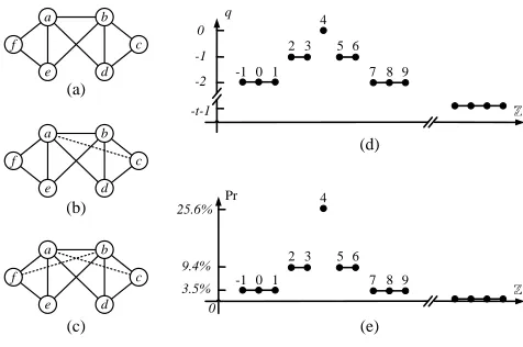
Figure 2: Examples of local sensitivity at distancet

indicate the magnitude of change of f when the connection be-tweeniandjis modified (added if absent; deleted if present) in the input graph. This then satisfiesLS(g) =maxi,jLSi j(g).

Although tempting, it is not correct to simply substituteLS(g)

forGSin the Laplace mechanism. This is becauseLS(g)itself con-veys information from the sensitive data. To address this problem, Nissim et al. [29] introducesmooth sensitivity, an upper bound of

LS(g), and show that differential privacy can be achieved by inject-ing Cauchy noise (instead of Laplace noise) calibrated to smooth sensitivity. As we show in Section 6, however, the adoption of Cauchy noise considerably degrades the quality of the output from a differentially private algorithm. This issue could be alleviated by combining smooth sensitivity with Laplace noise, but the resulting solution would only achieve a weakened version ofε-differential privacy (referred to as(ε,δ)-differential privacy [10]).

In this paper, we do not use smooth sensitivity, but adopt an in-termediate notion oflocal sensitivity at distance tas a crucial part of our solution.

DEFINITION2.4 (LOCALSENSITIVITY ATDISTANCEt[29]).

The local sensitivity of f at distance t is the largest local sensitivity attained on graphs at distance at most t from g. The formal definition is:

LS(g,t) = max

g∗_|_d₍_g,g∗₎_≤_tLS(g

∗₎_.

(5)

Note that LS(g,t)is a monotonically increasing function of t.

By analogy withLS(g,t)andLS(g), we further defineLSi j(g,t)as

the largestLSi j(·)attained on graphs at distance at mosttfromg.

ThenLS(g,t) =maxi,jLSi j(g,t).

Figure 2 gives an example of local sensitivity at distancet for triangle counting. The initial graphgin Figure 2(a) contains five nodes, three edges and no triangle. Its local sensitivity equals 1, achieved by adding edge(i,j)to the graph, i.e.,LS(g) =LSi j(g) =

1. Thereafter,LS(g,1)allows one extra modification before cal-culatingLS. In Figure 2(b), we show how the dashed edge(b,j)

affectsLSi j(·), makingLS(g,1) =LSi j(g,1) =2. Furthermore, we

find thatLScould never rise to 3 within 2 steps of modifications, and Figure 2(c) illustrates one example achievingLS(g,3) =3.

3. OVERVIEW OF SOLUTION

[image:5.612.320.546.53.138.2]

This section presents the steps for using our ladder framework for answering subgraph counting queries underε-differential pri-vacy, given an appropriate function with some assumed properties (these functions are instantiated and proved to possess these prop-erties in subsequent sections). Like the Laplace mechanism, we add a certain amount of noise to the true answer to prevent infer-ence of sensitive information. However, to achieve better results, we aim to exploit the fact that most realistic graphs can tolerate a lower amount of noise while still providing the needed privacy. Towards this end, we need to tailor the noise to the given input, without revealing anything about the input by our choice of noise distribution. We introduce how to build such a distribution through the exponential mechanism in Section 3.1, then give an algorithm for efficient sampling in Section 3.2.

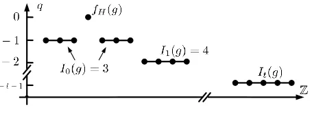
Figure 3: An example of a ladder quality

3.1 Building a Solution Distribution

Assume that we are given a queryfH(g)that counts the number

of subgraphsHing. Letηbe the distribution of the solution that we return as a private version of fH(g). In a nutshell,ηis a

dis-crete distribution defined over the integer domain, such thatη(k)

increases withq(g,k), whereq(g,k)≤0 is a non-positive integer that quantifies the loss of data utility when we publishkinstead of

fH(g). We refer toqas aquality function, since we will use it as a

quality function in the exponential mechanism. The expression of

η(k)as a function ofq(g,k)is given in equation (3) of Section 2.1. Our choice ofqis determined by a functionIt(g), which

de-fines howqvaries. Figure 3 gives a working example of theqand

It(g). In particular,qis a symmetric function over the entire

in-teger domain, centered at fH(g). We define the quality function

to take its maximum value at fH(g). Without loss of generality,

we setq(g,fH(g)) =0. For other possible answers, the quality

de-creases as the distance to the true answer inde-creases. The decreasing speed is controlled by functionIt(g). We refer to each quality level

(0,−1,−2, . . .) as arungof the ladder. In the figure, the first rung, corresponding to a quality level of−1, consists of theI0(g)integers on each side of fH(g), whose distances to fH(g)are no larger than

I0(g). The next rung is formed of the nextI1(g)integers on each side with quality−2, and so on. We say thatItgives the “width” of

thet+1st rung.

DEFINITION3.1 (LADDERQUALITY). Formally, given function It(g)we define the ladder quality function q(g,k)by

(i) q(g,fH(g)) =0;

(ii) ∀k∈fH(g)± ∑tu=−10It(g),∑

u

t=0It(g), set q(g,k) =−u−1.

After assigning each integer a quality score, we need to deter-mine the sensitivity of the quality function,

∆q= max

k,g,g0_|_d₍_g,g0₎_≤1|q(g,k)−q(g

0_,

k)|,

in order to apply the exponential mechanism. For arbitrary query class fHand functionIt(g), there is no simple answer: it can be the

case that∆qis unbounded. Consequently, we restrict our attention

to a class of well-behaved functionsIt(g)that we will refer to as

ladder functions. By analogy, we require that if we place two lad-ders corresponding to neighboring graphsg,g0next to each other and stand on thet’th rung ofg’s ladder, we can easily “leap across” tog0’s ladder, since the rung at the corresponding position is at al-most the same height. Formally,

PROPERTY3.1 (SMALL LEAP PROPERTY). The ladder

quality q(g,k)defined by It(g)has bounded∆q.

In Section 4, we give a class of functions that meet this property since they have a constant∆q=1. For now, we simply assume that ∆qis bounded and known to us, therefore, we can build the solution

(6)

Algorithm 1 NoiseSample(fH,g,ε,It): returnsf∗

1: Compute true answer fH(g);

2: range[0] ={fH(g)};weight[0] =1·exp

ε

2∆q·0

; 3: Initializedst=0;

4: fort=1 toMdo

5: range[t] =fH(g)±(dst,dst+It−1(g)]; 6: weight[t] =2It−1(g)·exp

ε

2∆q· −t

;

7: dst=dst+It−1(g); 8: end for

9: weight[M+1] =

2C·exp

ε

2∆q· −(M+1)

1−exp

− ε

2∆q

;

10: Sample an integert∈[0,M+1]with a probabilityweight[t]

over sum of weights; 11: ift≤Mthen

12: return a uniformly distributed random integer inrange[t]; 13: else

14: Sample an integerifrom the geometric distribution with pa-rameterp=1−exp− ε

2∆q

;

15: return a uniformly distributed random integer infH(g)±

{dst+i·C+ (0,C]}; 16: end if

3.2 Efficient Sampling from the Distribution

Our solution proceeds by using the ladder quality function to instantiate the exponential mechanism. This results in a solution which is guaranteed to provide differential privacy. However, the output of the mechanism can range over a very large, if not un-bounded, number of possibilities, which we must sample from. The naive approach of computing the probability associated with each output value is not feasible: there are too many to calculate. In-stead, we need a way to perform sampling in a tractable way. To reduce the time complexity of working with this infinite distribu-tion, we assume a convergence property ofIt(g), that there is a

“bottom rung” of our ladder below which all rungs are the same width.

PROPERTY3.2 (REGULAR STEP PROPERTY).It(g)

con-verges to a constant C within M steps, i.e., It(g) =C for any

t≥M.

With these two properties, we can more effectively use the expo-nential mechanism, since there is a bounded number of sampling probabilities. Algorithm 1 gives pseudocode for the sampling pro-cess under these assumptions, which we now explain. Our algo-rithm aggregates all integers with the same quality, say−t, ast’th rung. The range function (Line 5) describes the domain of each rung, and the weight function (Line 6) gives the sum of weights within the domain. We illustrate how to calculate the range and weight for the first few rungs, e.g., rung 0 (the center) to rungM

(Lines 2-8). For other rungs with indicest>M, we observe that their weights 2C·exp(ε/2∆q· −t)form a geometric sequence oft

with common ratio exp(−ε/2∆q). Therefore, we can write down a

closed form sum of weights for all remaining rungs, as in Line 9, considered as one large rung indexed byM+1.

Lines 10-16 perform the random sampling. First, one rung is sampled with a probability proportional to its weight. If it is rung

M+1, then we need to further specify the rung index by sampling from a geometric distribution (Line 14). At the end, we return a random integer within the range of the sampled rung as the final result. The time complexity of Algorithm 1 except Line 1 isO(M).

Privacy guarantee.The correctness of Algorithm 1 follows from the correctness of the exponential mechanism [25]. Therefore, we have the following theorem (proof in Appendix B).

THEOREM 3.1. Algorithm 1 satisfies ε-differential privacy, provided Ithas Properties 3.1 and 3.2.

4. LADDER FUNCTIONS

The previous section explains how to build and sample a solu-tion distribusolu-tion with Algorithm 1, given a suitable funcsolu-tionIt(g).

In what follows, we consider how best to define such functions in general; we then apply this insight for the functions of interest that count various types of subgraph in the next section.

Some requirements for a good function are as follows. It(g)

should be a function of input graphgand stept, such that (i)It(g)

satisfies Properties 3.1 and 3.2, to guarantee the correctness of Al-gorithm 1; (ii)It(g)is small. The rationale is thatIt(g)controls

the shape of the ladder. The smaller It(g)the faster the quality

decreases away from the true answer, and hence, the exponential mechanism tends to generate a distribution with higher probabili-ties for outputs closer to the true answer (smaller noise). In what follows, we first introduce a class ofladder functions, and give sev-eral examples. Then we prove that ladder functions always achieve a constant value for∆q, the sensitivity of the quality function

(pro-viding Property 3.1). Last, we construct a convergent ladder func-tion for subgraph counting queries which always converges to the global sensitivity within n₂

steps (meeting Property 3.2). We now formalize our notion of a ladder function.

DEFINITION4.1 (LADDERFUNCTION). It(g)is said to be a

ladder functionof query f if and only if

(a) LSf(g)≤I0(g), for any g;

(b) It(g0)≤It+1(g), for any pair of neighboring graphs g,g0, and

any nonnegative integer t.

A straightforward example of a ladder function is the constant functionIt(g) =GS, sinceLS(g)≤GSfor anyg, and a constant

always satisfies the second requirement. However, as discussed in Section 2.2,GScan be extremely large for subgraph counting, which does not adapt to typical graphs, which may not require so much noise. The local sensitivityIt(g) =LS(g) could be much

smaller thanGS, but unfortunately is not a ladder function because

LS(g0)≤LS(g)doesnothold for all pairs of neighboring graphs. Our insight for designing good ladder functions is that we can use a relaxation of local sensitivity instead. Specifically, we adopt the notion of local sensitivity at distancet, i.e.,LS(g,t). We now prove that this choice is optimal within our framework: local sensitivity at distancet is theminimum ladder function, i.e. it is the lower envelope of all possible ladder functions.

THEOREM 4.1. LS(g,t) is the minimum ladder function that satisfies LS(g,t)≤It(g)for any ladder function It(g).

PROOF. We first prove thatLS(g,t)is a ladder function. (i)LS(g) =LS(g,0)(meeting Definition 4.1(a));

(ii) {g∗|d(g0,g∗)≤t} is a subset of {g∗|d(g,g∗)≤t+1}, given a pair of neighboring graphs g,g0 such thatd(g,g0)≤1. Therefore, it meets Definition 4.1(b), since:

LS(g0,t) = max

g∗_|_d₍_g0_,g∗₎_≤_tLS(g

∗₎

≤ max

g∗_|_d₍_g,g∗₎_≤_t₊₁LS(g

∗_{) =}

(7)

Next we proveLS(g,t)is no larger than any ladder functionIt(g)

by induction ont.

Basis:whent=0,LS(g,0) =LS(g)≤I0(g)for allg;

Inductive step:suppose thatLS(g,t)≤It(g)holds for allg. It must

be shown thatLS(g,t+1)≤It+1(g)holds for allg. For any pair of neighboring graphsg,g0, we haveIt+1(g)≥It(g0)givenIt(g)is a

ladder function. Thus,It+1(g)≥maxg0_|_d₍_g,g0₎_≤1I_t(g0)holds for all

g. Then given the assumption thatLS(g,t)≤It(g)holds for allg,

It+1(g)≥ max

g0_|_d₍_g,g0₎_≤1It(g

0₎_≥ _max

g0_|_d₍_g,g0₎_≤1LS(g

0_,_t₎ _{by hypothesis}

= max

g0_|_d₍_g,g0₎_≤1_g∗_|_dmax₍_g0_,g∗₎_≤_tLS(g

∗₎

= max

g∗_|_d₍_g,g∗₎_≤_t₊₁LS(g

∗_{) =}

LS(g,t+1)

thus showing that indeedLS(g,t+1)≤It+1(g)holds for allg. By induction,LS(g,t)≤It(g)holds for allgand all nonnegativet.

LS(g,t)plays an important role in our framework. For certain subgraph counting queries, e.g., f4,fk?, it is the best ladder

func-tion that we can ever find. However, it is not always the preferred choice: as shown in Section 5,LS(g,t)can be very hard to com-pute for some queries. To tackle this problem, we will present how to construct an alternate ladder function (basically, a relaxation of

LS(g,t)) which is (i) computationally efficient and (ii) still much smaller thanGS.

4.1 Bounded

∆

q

This subsection proves the most important property of ladder functions, that they satisfy Property 3.1.

THEOREM 4.2. If It(g)is a ladder function then the resulting

quality function q has∆q=1.

PROOF. To prove this theorem, we must show that for any pair of neighboring graphsg,g0, and any integerk∈Z,|q(g,k)− q(g0,k)| ≤1 always holds. That is, the quality ascribed to provid-ingkas an output differs by at most 1 for neighboring graphs. In what follows, we discuss three different cases based on how close the value ofkis to the top of the ladder.

Special case 1, the center: k= fH(g)⇒q(g,k) =0. Given

the properties of local sensitivity and ladder function (Defini-tion 4.1(a))|k−fH(g0)| ≤LS(g0)andLS(g0)≤I0(g0), we have

fH(g0)−I0(g0)≤fH(g)≤ fH(g0) +I0(g0). (6) That is, sincekis the query answer for a neighboring graph of

g0, it must fall within the local sensitivity of the query answer for

g0. From Definition 3.1(i) and (ii) withu=0 we haveq(g0,k)∈ {0,−1}. Thus, the difference of quality is bounded by 1.

Special case 2, first rung:Ifk∈fH(g) + (0,I0(g)], thenq(g,k) = −1: kis on the first rung. By the construction of the ladder func-tion,q(g0,k)should be on the center, the first or the second rung, and so the quality changes by at most 1. Formally, the lower bound ofkas a function ofg0is

k>fH(g)≥ fH(g0)−I0(g0) (from (6)); and the upper bound is

k≤fH(g) +I0(g)≤ fH(g0) +I0(g0) +I1(g0),

using Definition 4.1(b) to showI0(g)≤I1(g0), combined with (6). Applying Definition 3.1, the value of the quality function satisfies

q(g0,k)∈ {0,−1,−2}, and so the bound holds.

General case: Consider k∈ fH(g) + (∑ut=−10It(g),∑ut=0It(g)] so

q(g,k) =−u−1, whereu>0—we are on theu+1st rung on the ladder forg. We argue that we can only climb or descend a single rung when we move to the ladder forg0. The lower bound onkas a function ofg0can be obtained using similar steps to case 2 above, from (6) andu−1 invocations of Definition 4.1(b):

k>fH(g) + u−1

∑

t=0

It(g) =fH(g) +I0(g) +

u−1

∑

t=1

It(g)

≥fH(g0) + u−2

∑

t=0

It(g0).

The upper bound uses a similar argument:

k≤fH(g) + u

∑

t=0

It(g)

≤fH(g0) +I0(g0) +

u+1

∑

t=1

It(g0) = fH(g0) + u+1

∑

t=0

It(g0).

Therefore,q(g0,k)is close toq(g,k) =u−1:

k∈fH(g0) + u−2

∑

t=0

It(g0), u+1

∑

t=0

It(g0)

#

⇒q(g0,k)∈ {−u,−u−1,−u−2}.

The analysis above proves the result for allk≥ fH(g). For

in-tegersk< fH(g), the proofs of special case 2 and the general case

are symmetric, and yield the required result.

4.2 Convergence

This subsection shows how to design aconvergentladder func-tion for subgraph counting queries that meets Property 3.2. First, we state a useful lemma for our subsequent analysis. The proof is immediate given the definition of ladder functions, so we omit it.

LEMMA 4.1. If f(g,t) and h(g,t) are ladder functions,

min(f(g,t),h(g,t))is a ladder function.

Using this result, one can easily design a convergent ladder function, e.g., min(It(g),GS), if the original functionIt(g)is

un-bounded. This is critical since Algorithm 1 requires a convergent function. UnlikeLS(g,t)which converges toGSnaturally, some ladder functions may need to be explicitly bounded byGS.

THEOREM 4.3. For any subgraph counting query fH,

min(It(g),GS) is a ladder function of fH that converges to GS

within n₂steps, given It(g)is a ladder function of fH.

PROOF. min(It(g),GS)is a ladder function: sinceIt(g)andGS

are both ladder functions we can invoke Lemma 4.1.

As the distance between any two graphs inGnis no larger than n

2

, we have that

g∗|d(g,g∗)≤ n₂ =Gn holds for any graph

g∈Gn. Thus, the local sensitivity at distance n2

equalsGS, i.e.,

LS g, n₂

= max

g∗_|_d₍_g,g∗₎_≤₍n

2)

LS(g∗) =max

g∗_∈G

n

LS(g∗) =GS.

GivenLS(g,t)is the minimum ladder function and is monotoni-cally increasing int, it followsIt(g)≥LS(g,t)≥LS g, n₂=GS

for anyt≥ n₂

. Hence, min(It(g),GS) =GSfor anyt≥ n₂.

Recall that the time complexity of Algorithm 1 (except Line 1) is linear inM. Therefore we can conclude that the algorithm ter-minates inO(n2)time for any subgraph counting query, if a ladder functionIt(g)is given in advance. Quadratic time can still be large,

(8)

5. APPLICATIONS

In this section, we show how to apply our framework for a va-riety of subgraph counting queries, includingf4,fk?,fkCand fk4.

LS(g,t)of the functionsf4and fk?are carefully studied in [17,29],

which can serve as ladder functions for these two queries directly. However, as we will show in this section, computingLS(g,t)can be hard for some queries, e.g.,fkCand fk4. Instead of usingLS(g,t), we present an efficient method to build a convergent upper bound ofLS(g,t), which is shown to satisfy the requirements in Defini-tion 4.1. Such an upper bound could be used as the ladder funcDefini-tion forfkCand fk4.

Graph statistics.Our detailed analysis of global sensitivity, local sensitivity and its upper bound rely on some simple graph statistics related to the (common) neighborhood of nodes.

DEFINITION5.1 (GRAPHSTATISTICS). Let(xi j)n×n be the

adjacency matrix of an undirected, simple graph on n nodes. xi j=

1when there exists an edge between nodes i and j,0otherwise. Let didenote the degree of node i, and dm=maxidibe the maximum

degree of the graph.

Let Ai j be the set of common neighbors of i and j. Node l

be-longs to Ai jif and only if xilxl j=1. Let ai j=|Ai j|be the number

of common neighbors of i,j, and am=maxi,jai jbe the maximum

number of common neighbors of a pair of nodes in the graph. Let bi j=di+dj−2ai j−2xi jdenote the the number of nodes connected

to exactly one of the two nodes i,j.

5.1 LS

(

g

,

t

)

as Ladder Function

Triangle counting. In Lemma 5.1, we give the global sensitivity and local sensitivity at distancetof triangle counting.

LEMMA5.1 (CLAIM3.13OF FULL VERSION OF[29]).

The global sensitivity of f4is GS=n−2; The local sensitivity at

distance t of f4is LS(g,t) =maxi,jLSi j(g,t), where

LSi j(g,t) =min

ai j+

_t₊_min₍_t_,_b

i j)

2

,n−2

.

It is easy to prove thatLS(g,t)converges toGSwhent≥2n. The time complexity of computingLS(g,t)fort∈[0,2n]isO(M(n)), whereM(n)is the time needed to multiply twon×nmatrices.

k-star counting.Another important problem of subgraph counting studied in [5, 17] isk-star counting. Lemma 5.2 shows its global sensitivity and local sensitivity at distancet.

LEMMA5.2 (LEMMA3.4OF[17]). The global sensitivity of fk? is GS=2n_k−2₋₁;The local sensitivity at distance t of fk? is

LS(g,t) =maxi,jLSi j(g,t), where

LSi j(g,t) =

    

    ¯

di+t k−1

+ d¯j k−1

, if t≤Bi;

n−2

k−1

+ d¯j+t−Bi k−1

, if Bi<t≤Bi+Bj;

2 n_k−2₋₁

, if Bi+Bj<t.

Hered¯i=di−xi jand Bi=n−2−d¯i.d¯jand Bjare defined

anal-ogously. Without loss of generality, assume that di≥dj.

As withf4,LS(g,t)of fk?converges toGSwhent≥2n. It takes

O(nlogn+m)time to computeLS(g,t)fort∈[0,2n].

5.2 Customized Ladder Function

AlthoughLS(g,t)works well for triangle andk-star counting, it cannot be extended to the class of queries whoseLS(g,t)are NP-complete to compute, e.g.,k-clique counting for a constantk>3

(the reduction is shown for completeness in Appendix A) andk -triangle counting fork>1 (proved in [17]). To address this prob-lem, the authors of [17] propose to use adifferentially private ver-sion of local sensitivity, to replace the inefficientLS(g,t). How-ever, this method is quite restricted because (i) it is specifically for

k-triangle counting; (ii) it achieves(ε,δ)-differential privacy only, andε is limited to(0,3₂ln3₂ ≈0.6]. In this section, we illustrate how to avoid usingLS(g,t)by designing a new customized ladder function.

5.2.1

k

-clique counting

We first emphasize that we are only interested in a small constant

khere, otherwise the counting queryfkCitself is hard to compute.

1- and 2-clique counting are trivial in our setting, and 3-clique (tri-angle) counting is already well addressed in Lemma 5.1. For other constantk>3, we aim to design a functionIt(g)which satisfies all

the requirements in Definition 4.1.

First of all, we introduce some building blocks ofIt(g), i.e.,am

(see Definition 5.1), and the global and local sensitivity of fkCin

the next lemma

LEMMA 5.3. The global sensitivity of fkCis GS=

n−2

k−2

;the local sensitivity of fkCis

LS(g) =max

i,j C(g(Ai j),k−2),

where g(S)denotes the subgraph induced on g by the node subset S, andC(g,k)is the number of k-cliques in graph g.

The global sensitivity is achieved when deleting one edge from a complete graph withnnodes. The local sensitivity at(i,j), i.e., C(g(Ai j),k−2), indicates the number of k-cliques that contain

nodesiand jwhen edge(i,j)is added.

Next we give our ladder function fork-clique counting in Theo-rem 5.1 and explain the intuition of this design in the proof.

THEOREM 5.1.

It(g) =min

LS(g) +

am+t

k−2

−

am

k−2

,GS

is a ladder function for fkC.

PROOF. By Lemma 4.1, we learn that provingLS(g) + a_km+₋₂t −

am k−2

is a ladder function is sufficient to prove this theorem. The proof contains the following three steps.

(1)LS(g)≤I0(g), for anyg. This step is trivial sinceI0(g) =LS(g); (2)I0(g0)≤I1(g), for any pair of neighboring graphsg,g0. LetAi j

(A0_{i j})be the set of common neighbors of nodesi,jing(g0). Letam

(a0_m)be maximum number of common neighbors ing(g0). Note that the size ofAi jis bounded byam.

LS(g0)−LS(g) =max

i,j C(g

0₍_A0

i j),k−2)−max_i,_j C(g(Ai j),k−2)

≤max

i,j C(g

0₍_A0

i j),k−2)−C(g(Ai j),k−2)

.

Recall that there is only one edge difference betweengandg0. To increase the number of(k−2)-cliques ing(Ai j)by editing one

edge, one can either (i) add one edge withing(Ai j)while keeping

the setAi j unchanged, or (ii) expand Ai j by one new node. The

maximum increase, i.e., am k−3

is achieved in the case thatg(Ai j)is

a complete graph of sizeamandg0(A0i j)is a complete graph of size

am+1. However, observe that since

am

k−3

=

am+1

k−2

−

am

(9)

we have

LS(g0)≤LS(g) +

am+1

k−2

−

am

k−2

⇔ I0(g0)≤I1(g).

(3)It(g0)≤It+1(g), for any neighboring graphsg,g0 and integer

t>0. We make use of the combinatorial identity∑nk=0

k m

= _mn+₊1₁ and obtain

LS(g0) +

a0m+t

k−2

−

a0m

k−2

=LS(g0) +

t−1

∑

i=0

a0m+i

k−3

≤LS(g) +

am

k−3

+

t−1

∑

i=0

am+i+1

k−3

=LS(g) +

t

∑

i=0

am+i

k−3

=LS(g) +

am+t+1

k−2

−

am

k−2

,

which is equivalent toIt(g0)≤It+1(g). The central step of the proof relies on an important property of the maximum number of com-mon neighbors: its global sensitivity equals 1. So it holds that

a0m−am≤1, and so a

0

m+i k−3

≤ am+i+1 k−3

.

This ladder function converges toGS whent≥n. The major computational overhead ofIt(g)fort∈[0,n]isLS(g), which can

be computed withinO(nk)time via exhaustive search. In our exper-iment, we implement a sophisticated algorithm which utilizes the sparsity of the input to improve efficiency. It returnsLS(g)within a few seconds for all graphs tested in the next section.

5.2.2

k

-triangle counting

Besidesk-clique counting, we also presentk-triangle counting as another example of using customized ladder function. We state the currently known results aboutk-triangle counting as Lemma 5.4.

LEMMA5.4 (LEMMA4.1AND4.2OF[17]). The global sensitivity of fk4 is GS = n−2k

+2(n−2) n_k−3₋₁

. The local sensitivity of fk4is

LS(g) =max

i,j

ai j

k

+

_∑

l∈Ai j

ail−xi j

k−1

+

al j−xi j

k−1 !

;

We also have LS(g0)≤LS(g) +3 am k−1

+am _ka₋₂m,given a pair of

neighboring graphs g and g0.

Similarly, one can design a ladder function fork-triangle count-ing, as shown in Theorem 5.2. The proof follows the same lines as that of Theorem 5.1.

THEOREM 5.2.

It(g) =min LS(g) + t−1

∑

i=0

U(am+i),GS

!

is a ladder function for fk4, where U(a) =3 k−1a

+a _k₋₂a

.

It takest≥3nsteps for this ladder function to converge toGS, and the time complexity of computingIt(g)fort∈[0,3n]would be

O(n3)using a naive method.

To summarize, we observe some similarities betweenk-clique andk-triangle counting. First, theirLS(g,t)functions are both NP-complete to compute, which motivates our customized ladder func-tions. Second, there exist efficient ways to compute the local sen-sitivitiesLS(g), andLS(g0)−LS(g)is bounded by a function of a variable whose global sensitivity is constant, e.g.,amordm. Any

subgraph counting query with these two properties could be pro-cessed by our framework with a customized ladder function as in Theorems 5.1 and 5.2.

6. EXPERIMENTS

6.1 Experimental Settings

[image:9.612.55.292.140.221.2]

Datasets.We make use of six real-world graph datasets in our ex-periments: AstroPh, HepPh, HepTh, CondMatandGrQcare collaboration networks from the e-print arXiv, which cover scien-tific collaborations between authors who submitted papers to As-tro Physics, High Energy Physics, High Energy Physics Theory, Condensed Matter and General Relativity categories, respectively. In particular, if a paper is co-authored bykauthors, the network generates a completed connected subgraph (k-clique) onknodes representing these authors. Enronis an email network obtained from a dataset of around half a million emails. Nodes of the net-work are email addresses and if an addressisent at least one email to address j, the graph contains an undirected edge fromito j. Tabel 2 illustrates the properties of the datasets and their results to four subgraph counting queries. All datasets can be downloaded from Stanford Large Network Dataset Collection [21].

Baselines. To justify the performance of our algorithm (denoted as Ladder) in answering subgraph counting queries, we compare it with other four approaches: (i) Laplace [11], which directly injects Laplace noise with scaleGS/ε to the true subgraph counts. (ii)

Smooth [17, 29], which first computes a smooth upper boundSS

of the local sensitivity, then adds Cauchy noise scaled up by a fac-tor of 6SS/εto the answer. It is only evaluated on two queries f4 and fk?due to the hardness of computingSSforfkCand fk4. (iii) NoisyLS [17], which achieves differential privacy by adding noise proportional to adifferentially privateupper bound on local sensi-tivity (instead of the smooth upper bound used in Smooth). This ap-proach is designed forfk4, and is the only(ε,δ)-differentially pri-vate baseline algorithm. The parameterεis restricted to(0,3₂ln2₃]

whileδ is set to a fixed value 0.01 in our experiments. (iv) Re-cursive [5], which answers the query by releasing a differentially private lower bound (which has low-sensitivity) of the counting result. The time complexity of this algorithm is super-quadratic to the number of subgraphs. All experiments using the Recursive mechanism failed to complete within 4 days except for two cases:

HepTh-4andGrQc-4since their counting results are relatively

small. In contrast, all local sensitivity based solutions (i.e., Ladder, Smooth, NoisyLS) are rather efficient, and in fact share the same time complexity.

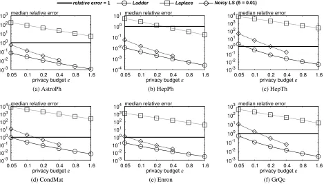
Evaluation.We evaluate the performance of Ladder and four base-lines on four subgraph counting queries over all six datasets. We measure the accuracy of each method by themedian relative er-ror[17], i.e., the median of the random variable|A(g)−f(g)|/f(g)

whereA(g)is the differentially private output and f(g)is the true answer. The reason of choosing this measurement is that the mean of Cauchy noise (used in Smooth) is undefined. In other words, the mean error of the Smooth method is never stable, no matter how large the sampling set is. Therefore, in accordance with prior works [5, 17], we choose to report median error. We also include a bold line to indicate a relative error of 1. Any result above this line is of no practical value. For each result reported, we repeat each experiment 10,000 times to get the median, except for Recursive (where we perform 100 repetitions).

6.2 Counting Queries

(10)

[image:10.612.65.539.68.440.2]

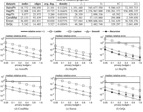
Table 2: Datasets properties

datasets nodes edges avg. deg. density 4 3? 4C 24

AstroPh 18,772 198,050 21.101 0.1124% 1,351,440 545,677,550 9,580,415 72,355,715

HepPh 12,008 118,491 19.735 0.1644% 3,358,499 1,276,967,000 150,281,372 936,890,335

HepTh 9,877 25,975 5.260 0.0533% 28,339 2,098,336 65,592 429,013

CondMat 23,133 93,439 8.078 0.0349% 173,361 37,115,060 294,008 2,349,650

Enron 36,692 183,831 10.020 0.0273% 727,044 4,909,606,844 2,341,639 36,528,276

GrQc 5,242 14,485 5.527 0.1054% 48,260 2,482,748 329,297 2,041,499

relative error = 1 Ladder Laplace Smooth Recursive

10-4 10-3 10-2 10-1 100

0.05 0.1 0.2 0.4 0.8 1.6 privacy budget ε

median relative error

10-4 10-3 10-2 10-1 100

0.05 0.1 0.2 0.4 0.8 1.6 privacy budget ε

10-3 10-2 10-1 100 101

0.05 0.1 0.2 0.4 0.8 1.6 privacy budget ε

(a) AstroPh (b) HepPh (c) HepTh

10-4 10-3 10-2 10-1 100 101

0.05 0.1 0.2 0.4 0.8 1.6 privacy budget ε

10-4 10-3 10-2 10-1 100

0.05 0.1 0.2 0.4 0.8 1.6 privacy budget ε

10-3 10-2 10-1 100 101

0.05 0.1 0.2 0.4 0.8 1.6 privacy budget ε

(d) CondMat (e) Enron (f) GrQc

Figure 4: Triangle counting

Triangle counting.The first query that we evaluate is the triangle countingf4(see Figure 4). In summary, Ladder achieves good ac-curacy on f4over all datasets. When privacy budget is relatively large, e.g.,ε=1.6, its median relative error always stays below or close to 0.1%. With the decrease ofε, the accuracy drops but it is

still smaller than 10% even whenε=0.05. Compared with other

differentially private methods, Ladder clearly outperforms Laplace and Smooth in all cases, simply because it injects less noise to the true results. The improvement is significant since the y-axis in shown on a log scale. As for Recursive, it is rather competitive whenεis small, sayε≤0.1. However, the gap between Recursive and Ladder begins to grow whenε increases. To explain, recall

that the error of Recursive comes from two parts: bias of the lower bound and noise injected to the lower bound. Asεincreases, the scale of noise reduces, while the bias is less sensitive to the change ofεthen becomes the dominating factor of the error.

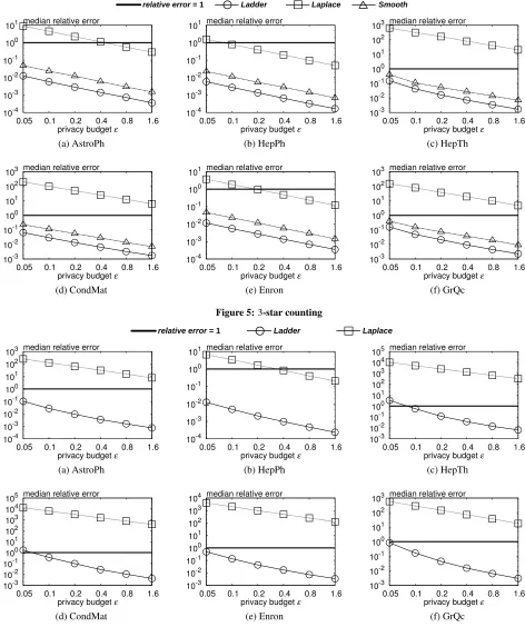
k-star counting. Next we evaluate different methods for 3-star counting f3? in Figure 5. Ladder keeps returning extremely

ac-curate results for largeε, and reasonably good results for smallε. Meanwhile, it is still the best solution with anε-differential privacy guarantee in all settings. In contrast to the case of triangle count-ing, the performance of Laplace degrades significantly compared to other two local sensitivity based solutions. The main reason is that

GSof triangle counting is linear tonwhile that of 3-star counting is quadratic. On the other hand, the counting results do not increase so dramatically due to the locality of inputs. Therefore the relative error of Laplace increases. Local sensitivity, however, can capture the locality of inputs, leading to a stable relative error when the query is changed.

k-clique counting.Figure 6 presents the results of 4-clique count-ing (f4C). Ladder is the only private solution besides the naive

Laplace, and the former is orders of magnitude better than the lat-ter in lat-terms of accuracy. The lines of Ladder always stay below the bold lines except for two points whereε is extremely small,

and the gaps increase markedly withε. In contrast, the quality of results from Laplace tends to be rather poor, if it is usable at all. Thus we conclude that Ladder is the only effective and efficient algorithm for releasing privatek-clique counting.

(11)

relative error = 1 Ladder Laplace Smooth

10-4 10-3 10-2 10-1 100 101

0.05 0.1 0.2 0.4 0.8 1.6 privacy budget ε

10-4 10-3 10-2 10-1 100 101

0.05 0.1 0.2 0.4 0.8 1.6 privacy budget ε

10-3 10-2 10-1 100 101 102 103

0.05 0.1 0.2 0.4 0.8 1.6 privacy budget ε

10-3 10-2 10-1 100 101 102 103

0.05 0.1 0.2 0.4 0.8 1.6 privacy budget ε

10-4 10-3 10-2 10-1 100 101

0.05 0.1 0.2 0.4 0.8 1.6 privacy budget ε

10-3 10-2 10-1 100 101 102 103

0.05 0.1 0.2 0.4 0.8 1.6 privacy budget ε

[image:11.612.63.535.56.620.2]

Figure 5:3-star counting

relative error = 1 Ladder Laplace

10-4 10-3 10-2 10-1 100 101 102 103

0.05 0.1 0.2 0.4 0.8 1.6 privacy budget ε

10-4 10-3 10-2 10-1 100 101

0.05 0.1 0.2 0.4 0.8 1.6 privacy budget ε

10-3 10-2 10-1 100 101 102 103 104 105

0.05 0.1 0.2 0.4 0.8 1.6 privacy budget ε

10-3 10-2 10-1 100 101 102 103 104 105

0.05 0.1 0.2 0.4 0.8 1.6 privacy budget ε

10-3 10-2 10-1 100 101 102 103 104

0.05 0.1 0.2 0.4 0.8 1.6 privacy budget ε

10-3 10-2 10-1 100 101 102 103

0.05 0.1 0.2 0.4 0.8 1.6 privacy budget ε

Figure 6:4-clique counting

NoisyLS. In summary, Ladder is a more preferable solution for pri-vatek-triangle counting.

Average degree and density.Besides the comparison among pri-vate algorithms, we are also interested in the impact of input graphs to the private counting results. Intuitively, a graph with more edges (assuming a fixed number of nodes) is likely to have more copies

(12)

relative error = 1 Ladder Laplace Noisy LS (δ = 0.01)

10-3 10-2 10-1 100 101 102 103

0.05 0.1 0.2 0.4 0.8 1.6 privacy budget ε

10-4 10-3 10-2 10-1 100 101

0.05 0.1 0.2 0.4 0.8 1.6 privacy budget ε

10-3 10-2 10-1 100 101 102 103 104

0.05 0.1 0.2 0.4 0.8 1.6 privacy budget ε

10-3 10-2 10-1 100 101 102 103 104

0.05 0.1 0.2 0.4 0.8 1.6 privacy budget ε

10-3 10-2 10-1 100 101 102 103 104

0.05 0.1 0.2 0.4 0.8 1.6 privacy budget ε

10-3 10-2 10-1 100 101 102 103

0.05 0.1 0.2 0.4 0.8 1.6 privacy budget ε

[image:12.612.68.537.56.329.2]

Figure 7:2-triangle counting

have better overall accuracy. Interestingly, local sensitivity based algorithms like Ladder and Smooth also benefit notably from high density inputs, implying that local sensitivity does not increase as drastically as the counting results as the graph gets denser.

6.3 Stochastic Kronecker Models

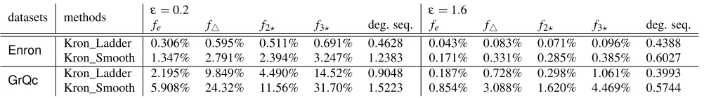
To further justify the importance of subgraph counts, we show how accurate counts lead to accurate graph models. Here we adopt the stochastic Kronecker model [20], a sophisticated method which can simulate large real-world graphs with only a few parameters. The algorithm in [13, 26] provides a way to estimate parameters of the simplest Kronecker model from a small set of subgraph counts:

fe(the number of edges),f4,f2?andf3?. Therefore, one can easily

build a Kronecker model then generate synthetic Kronecker graphs with differential privacy guarantees, if provided fourprivatecounts in advance. We aim to evaluate how the noise in private counts affects the accuracy of Kronecker models. In this set of experi-ments, we build three types of Kronecker models: (i) Kron-True is a non-private model, and tuned from the true subgraph counts of the graph; (ii) Kron-Ladder satisfiesε-differential privacy. The

privacy budgetεis split into four parts equally, and each is used to generate a private subgraph count. The Laplace mechanism is effective enough to release fesince it has a constantGS=1. For

f4, f2?and f3?, we employ Ladder. (iii) Kron-Smooth is

identi-cal to Kron-Ladder except thatf4, f2?and f3?are released by the

Smooth mechanism.

To measure the distortion of Kron-Ladder from Kron-True, we look into the difference of their synthetic graphs. For Kron-True, we simply sample 100 synthetic graphs from the model. However, given that Ladder is a stochastic process, we first generate 100 independent Kron-Ladder models, and from each we sample 100 graphs. Therefore, Kron-Ladder is represented by a set of 10,000 graphs. Then the error between each pair of graphs from these two sets is measured, and an aggregate value is reported as the final

re-sult. The evaluation of Kron-Smooth follows the same procedures. We report the error of five graph queries including median relative error of fe, f4, f2?, f3?and average Euclidian error of the sorted

degree sequence (as in [15]).

Table 3 shows the empirical results with two datasets (Enron

and GrQc) and two privacy budgets (ε=0.2 and 1.6).

Kron-Ladder outperforms Kron-Smooth by considerable margins in all settings, which implies that Kron-Ladder generates more accurate Kronecker models. It is interesting to observe that the synthetic graphs of Kron-Ladder perform better in answering fe(recall that

both methods use Laplace mechanism forfe). Note that the

param-eter estimation algorithm [13, 26] is designed to find a Kronecker model that fitsallcounts well. Hence the noise in any count could affect the choice of Kronecker model, then introduce bias to other properties of the synthetic graphs. This explains how the large scale of noise inf4, f2?and f3?propagates to fein Kron-Smooth.

7. RELATED WORK

The question of being able to release information on graphs in a privacy-preserving way has been of interest for a number of years, driven by recent efforts around privacy-preserving data publishing. It is interesting to note that within the computer science community, the recent slew of interest in graph anonymization began with pub-lications that emphasized the difficulty of this problem. Backstrom

et al.[2] showed that an adversary could easily learn neighborhood information of targeted nodes from a “deidentified” (unlabeled) re-leased graph, if they could insert a small number of edges. Hay

(13)

[image:13.612.55.556.73.143.2]

Table 3: Accuracy of Kronecker models tuned from noisy counts

datasets methods ε=0.2 ε=1.6

fe f4 f2? f3? deg. seq. fe f4 f2? f3? deg. seq.

Enron Kron_Ladder 0.306% 0.595% 0.511% 0.691% 0.4628 0.043% 0.083% 0.071% 0.096% 0.4388

Kron_Smooth 1.347% 2.791% 2.394% 3.247% 1.2383 0.171% 0.331% 0.285% 0.385% 0.6027

GrQc Kron_Ladder 2.195% 9.849% 4.490% 14.52% 0.9048 0.187% 0.728% 0.298% 1.061% 0.3993

Kron_Smooth 5.908% 24.32% 11.56% 31.70% 1.5223 0.854% 3.088% 1.620% 4.469% 0.5744

The response of the research community to these demonstrations of the weakness of deidentification was the design of numerous methods which aimed to be more robust to attack. Drawing in-spiration from concurrent efforts onk-anonymity for tabular data, several approaches aimed to modify the input graph structure to produce an output graph that was not susceptible to the techniques used to defeat deidentification. Of particular note was the work of Liu and Terzi [23] which aimed to make graphsk-degree anony-mous, so that an adversary possessed of the knowledge of the de-gree of a target node would find at leastknodes in the released graph sharing that degree. Many subsequent works built on this foundation by proposing stronger structural requirements on the re-leased graph. Zhou and Pei [37] considered graphs with nodes of certain types, and sought to ensure that for every set of neighbor-hood links around a target node, there are multiple possible matches in the released graph. Zouet al.[38] proposedk-automorphism, re-quiring that every node in the released graph has at leastk−1 struc-turally indistinguishable counterparts (i.e. have the same pattern of links between neighbors, and neighbors-of-neighbors, etc.). A par-allel set of works were based on “clustering” within graphs, where groups of nodes are replaced by a “cluster” in the output graph, and only aggregate statistics of the cluster are revealed [6, 16, 34].

A survey of the state of the art in 2008 provides a snapshot of several dozen contributions in this area; in the intervening years that have been many more efforts in this direction. Nevertheless, a number of criticisms of this philosophy towards data anonymiza-tion have emerged. Principal amongst these is that methods which seek to prevent a specific attack by an adversary with a certain type of information and an assumed approach to reasoning are not ro-bust against “real-world” adversaries, who can bring unanticipated knowledge and inference techniques to circumvent these. Secon-darily, there is the perception that these methods provide only ad hoc rather than principled guarantees, and do not adequately pre-serve utility for their inputs. Instead, there has been growing in-terest in ways to provide a more formal guarantee of privacy. The main such model is Differential Privacy, which is not without its critics or identified limitations, but which nevertheless represents the current focus of efforts to provide workable privacy solutions.

Differential privacy [7] is rigorously formulated based on statis-tics and offers an extremely strong privacy protection. A plethora of efforts has been made to apply differential privacy to a broad range of problems. It is beyond the scope of this paper to give full coverage of all differential privacy methods; instead, see recent surveys [8,9,12,30] and references therein. A brief survey of differ-entially private algorithms for releasing subgraph counts is given in Section 1.2. In what follows, we review some other related efforts to realize privacy protection for graph data.

Hay et al. [15] translated the language of differential privacy to the graph context, and give the formal definitions of edge and node differential privacy. This paper and subsequent related ap-proaches [18,22] provide effective solutions to releasing the degree sequence of a sensitive graph, and use some sophisticated post-processing techniques to reduce noise. Proserpio et al. [31] and Sala et al. [33] further extend the problem to higher-order joint

degree sequences, which model more detailed information within the sensitive graph. A later work by Wang and Wu [35] improves Sala’s solution by calibrating noise based on smooth sensitivity, rather than the large global sensitivity. Moreover, the authors il-lustrate that synthetic graphs generated from the noisy joint degree sequence have a series of appealing properties. In addition, Mir and Wright [26] show how to bridge differentially private subgraph counts with Kronecker graph models, providing another method to generate synthetic graphs with privacy guarantees. In a differ-ent vein, [1, 14, 36] investigate differdiffer-entially private spectral analy-sis (e.g., singular value decomposition and random projection) for graph data. Their results imply a great potential to process/release large scale sensitive graphs like the Facebook friendship graph and call/SMS/email networks. Recently, Lu and Miklau [24] describe the use of a chain mechanism to release alternatingk-star andk -triangle counting with an (ε,δ)-differentially private guarantee. They also show how the published counts can be used to estimate the parameters of exponential random graph models.

The above discussion principally focuses on methods that pro-vide edge differential privacy, where two graphs are considered neighbors if they differ only in the presence of a single edge. There is also a branch of work studying other variants of graph differ-ential privacy. For example, [3, 5, 19] are the first few methods to providenodedifferential privacy with non-trivial utility guarantees. Node differential privacy is a qualitatively stronger privacy guaran-tee than edge differential privacy, where two graphs are considered neighbors if they differ in the presence of a node and all its in-cident edges. As a consequence, it generally requires substantially more noise to protect the released information. Meanwhile, Rastogi et al. [32] consider a relaxed version of edge differential privacy, called edgeadversarialprivacy, which relies on some assumptions about prior knowledge of the malicious user. As those assumptions might plausibly be violated in practice, this new definition actually provide less privacy assurance, compared to the conventional edge differential privacy.