Coupling methods for 2D/1D shallow water flow models for flood simulations

warwick.ac.uk/lib-publications

A Thesis Submitted for the Degree of PhD at the University of Warwick

Permanent WRAP URL:

http://wrap.warwick.ac.uk/88277

Copyright and reuse:

This thesis is made available online and is protected by original copyright.

Please scroll down to view the document itself.

Please refer to the repository record for this item for information to help you to cite it.

Our policy information is available from the repository home page.

Coupling Methods for 2D/1D Shallow Water Flow

Models for Flood Simulations

by

Chinedu Nwaigwe

Thesis

Submitted to the University of Warwick

for the degree of

Doctor of Philosophy

Centre for Scientific Computing

Contents

List of Tables v

List of Figures vi

Acknowledgments xii

Abstract xiii

Abbreviations xiv

Chapter 1 Introduction 1

1.1 Introduction . . . 1

1.2 Flood Flow Simulation . . . 3

1.3 The Main Ideas in Coupling Channel and Floodplain Flow Models . 4 1.4 Research Objectives . . . 6

1.5 Review of Coupling Methods . . . 8

1.6 Outline of the Thesis . . . 12

Chapter 2 Mathematical Models for Flood and Channel Flows 14 2.1 Introduction . . . 14

2.2 The Free-Surface Euler Equations . . . 15

2.2.1 Background . . . 15

2.2.2 Deriving the free-surface Euler Equations . . . 16

2.3 Derivation of 2D Shallow Water Equations . . . 18

2.4 1D Saint Venant Equations for an Open Channel With Varying Width 21 2.4.1 Background . . . 22

2.4.2 Deriving the SVM . . . 24

2.4.3 Locally Rectangular Channel . . . 29

2.4.4 1D Shallow Water Equations . . . 29

2.5.1 Hyperbolic PDEs . . . 30

2.5.2 Hyperbolic Conservation Laws . . . 30

2.5.3 Hyperbolicity of the Derived Models . . . 32

2.5.4 Properties of hyperbolic PDEs . . . 33

Chapter 3 Finite Volume Schemes For Free-Surface Flow Problems 36 3.1 Introduction . . . 36

3.2 Conservative Numerical Schemes . . . 38

3.3 Finite Volume Methods for Conservation Laws . . . 40

3.4 Finite Volume Method for the Flood Model . . . 41

3.4.1 The 2D Shallow Water Equations without Source Terms . . . 41

3.4.2 The 2D Shallow Water Equations with Bottom Topography . 44 3.4.3 The 2D Shallow Water Equations with Bottom Topography and Friction . . . 46

3.5 Finite Volume Method for the Channel Flow Model . . . 47

3.6 Boundary Conditions . . . 50

3.6.1 Solid Boundary . . . 51

3.6.2 Open Boundary . . . 51

3.7 Time step calculations . . . 52

3.8 Numerical Results . . . 53

3.8.1 Test Cases for the 1D Channel Flow Solver . . . 53

3.8.2 Test Cases For the 2D Floodplain Flow Solver . . . 57

3.8.3 Why Coupling is needed . . . 63

Chapter 4 The Horizontal Coupling Method 68 4.1 Introduction . . . 68

4.2 The Channel Model with Coupling Terms . . . 69

4.2.1 Notational Simplification . . . 74

4.2.2 Lateral Discharge Model During Flooding . . . 77

4.2.3 Summary of the Channel Flow Model for the HCM . . . 77

4.3 Floodplain Flow Model . . . 78

4.4 Summary of all Models in the HCM . . . 78

4.5 Numerical Implementation of the HCM . . . 78

4.5.1 Numerical Scheme for the Channel Flow Model . . . 79

4.5.2 1D SVM with Coupling Term . . . 80

4.5.3 Approximating Channel Lateral Discharge . . . 81

4.5.4 Discrete Coupling Terms . . . 84

4.5.6 Summary of the Schemes for the Horizontal Coupling Method 87

4.6 Properties of the HCM . . . 87

4.7 Implementation Strategy . . . 89

4.7.1 Black Box Solver stage . . . 90

4.7.2 Post-Processing Stage . . . 90

4.8 Numerical Results . . . 91

Chapter 5 The Vertical Coupling Methods (VCM) 95 5.1 Introduction . . . 95

5.2 Background . . . 97

5.2.1 Fundamental Equations . . . 102

5.2.2 Defining the layers . . . 103

5.3 The Lower Layer Models . . . 105

5.3.1 Mass Conservation Equation for Lower Layer . . . 105

5.3.2 Momentum Equation for Lower Layer . . . 109

5.3.3 Summary of Lower layer Models . . . 110

5.4 The Upper Layer Models . . . 110

5.5 Summary of the Channel Flow Model in the VCM . . . 111

5.6 Numerical Implementation of the VCM . . . 113

5.6.1 Introduction . . . 113

5.6.2 Background . . . 114

5.6.3 Step 1: Distribution of Full 2D data into two-layer data . . . 120

5.6.4 Step 2: Operator Splitting Method For Sub-Layer Models . . 121

5.6.5 Step 3: Updating full 2DdataH_i,jn+1,q_x,i,jn+1andq_y,i,jn+1forTi,j ∈Ki126 5.6.6 Finite Volume Methods for the intermediate solutions . . . . 129

5.6.7 Solution of the Upper Layer Model without Exchange Terms 129 5.6.8 Solution of the Lower Layer Model without Exchange terms 130 5.7 Desirable Properties of the VCM Scheme . . . 131

Chapter 6 Numerical Results for Coupling Methods 139 6.1 Introduction . . . 139

6.2 Test case 1 . . . 141

6.3 Test case 2 : Channel Flow into Elevated 2D Floodplain . . . 142

6.4 Test case 3 : Flooding of an initially dry floodplain . . . 146

Chapter 7 Summary, Conclusion and Recommendations 158 7.1 Summary . . . 158

7.3 Recommendation for further study . . . 160

Appendix A Numerical Flux Functions 162 A.1 Godunov-Type Finite Volume Schemes . . . 162

A.2 Approximate Riemann Solvers . . . 163

A.2.1 Roe Solver . . . 163

A.2.2 HLL Approximate Riemann Solver . . . 168

A.2.3 HLLC Approximate Riemann Solver . . . 169

List of Tables

3.1 Experimental Order of Convergence for the 1D Riemann Problem (1D test case 1). EA, EQ are the errors in the cross sectional area,

A and discharge, Q respectively, while EOCA and EOCQ are their

respective orders of accuracy. . . 56 3.2 Experimental Order of convergence for the 2D scheme using the flow

in parabolic basin problem (2D test 2). EH, Eqx and Eqy are the

errors in l1-norm of H, qx and qy respectively, while EOCH, EOCqx

and EOCqy are their respective experimental order of convergence. . 61

4.1 Grid cells, simulation times and number of time steps after ten sec-onds. . . 91

6.1 Grid cells, simulation times and number of time steps for Test 1.

Shows the grid used for each simulation method and the number of time steps and processor time taken to complete the simulation. . . 142

6.2 Grid cells, simulation times and number of time steps : Test 2. Shows

the grid used for each simulation method and the number of time steps and processor time taken to complete the simulation. . . 146

6.3 Grid cells for test case 3 showing the grids used for the floodplains

List of Figures

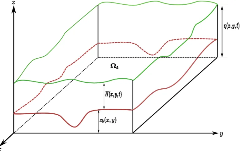
1.1 Shallow water flow over a domain with bottom topography zb(x, y)

(in red) comprising of a channel and floodplain. The length of the

channel is along the x-axis and the width, along the y-axis. The

water depth isH(x, y, t) and the free surface elevation isη(x, y, t) (in green). Symboltis time variable and (x, y, z)∈_R3_{. . . . 4}

1.2 Cross section at a fixed pointx in the flow domain depicted in figure 1.1. The bottom topography (in red) comprises of the channel in the

regionya ≤y ≤yb and the floodplain which occupies the remaining

regions. The free surface elevation is in green and H(x, y, t) is the water depth. . . 5

1.3 Cross section at a fixed x in the flow domain showing the different

regions for channel and the floodplains. The middle region is the channel which occupies the region ya ≤ y ≤ yb while the left and

right regions are the floodplains. . . 5

1.4 A picture of the different models for the different regions. The 2D shallow water equations for the floodplain flow (left and right) and a

channel flow model for the channel region (middle). . . 6

1.5 Flow cross section depicting only the channel region (channel cross section). Channel model is derived for the flow in this region. The

flow in the floodplains are used as boundary conditions. The channel

flow also serve as boundary conditions for the 2D floodplain models. 7 1.6 Channel flow structure for the horizontal coupling method (left) and

the vertical coupling method (right). . . 7

2.1 Shallow water flow over a domain with bottom topography zb(x, y)

(in red). The water depth isH(x, y, t) and the free surface elevation

2.2 Non-full channel flow cross section showing the left and right bank

elevations zbl(x) and zbr(x), the laterally flat free-surface elevation

¯

η(x, t) (in green), the bottom elevation in 2D zb(X~ ) (in red), the

width, B(x, z) of the channel at elevation, z above the reference

ele-vation z= 0, and the y−coordinates, yl(x, z) and yr(x, z) of the left

and right lateral walls at elevationz. . . 22

3.1 Discretization of the 1D domain [xa, xb] ⊂ R into N + 1 grid cells. Ki = [xi−1/2, xi+1/2] is the i-th cell, for i = 0,1,2, ..., N. xi =

xi−1/2+xi+1/2

2 and ∆xi =xi+1/2−xi−1/2 are center and width of Ki

respectively. . . 37

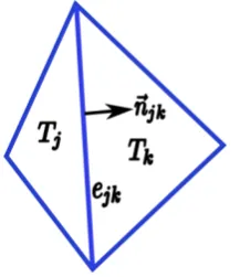
3.2 2D mesh showing two neighbour cells,Tj andTk, the edgeejkbetween

them and the normal vector~njk. . . 42

3.3 Exact and Numerical Results for the Riemann problem showing the

free surface elevation (left column) and velocity (right column) at different time steps. From the top to the bottom are the results at

the 100th, 200th, 400th and the last (465th) time steps. In each plot, the exact and numerical solutions are in blue and magenta respectively. 55

3.4 The channel width and bed variations for the 1D flow in varying

geometry channel. . . 57 3.5 Numerical Solution for the flow in channel with varying geometry (1D

test 2). . . 57

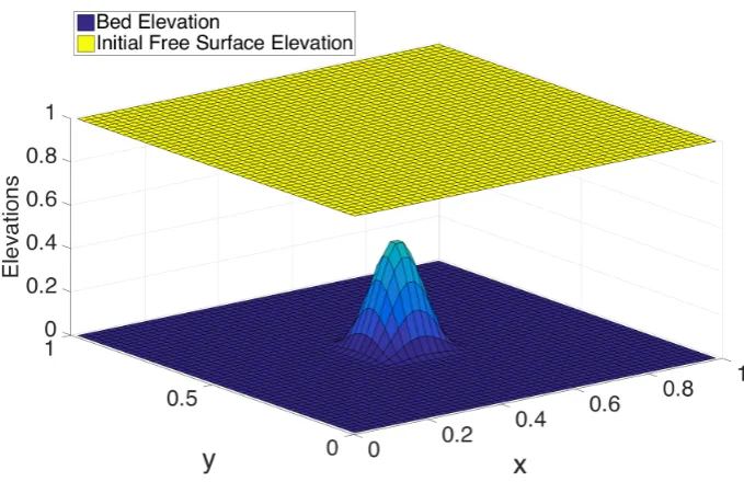
3.6 Bed elevation and initial free surface elevation for still water . . . 58 3.7 Numerical Results after 5 seconds for the still water over complex

bottom topography . . . 59

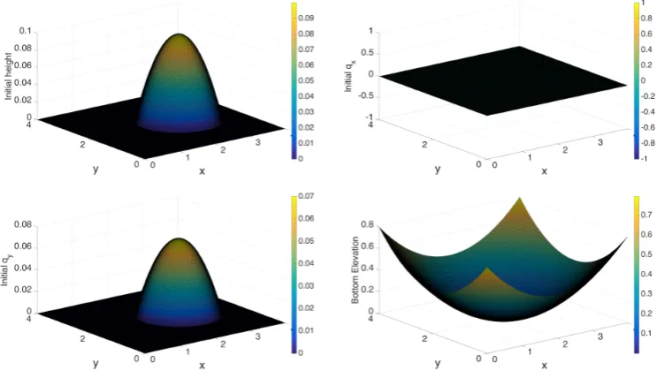
3.8 The bottom elevation and the initial water depth and discharges for 2D test case 2. . . 61

3.9 Numerical (left) and analytical (right) results for the water height

and the discharges after 5.93018 seconds for 2D test case 2. . . 62 3.10 Top view of Channel and Floodplain for river-flooding problem . . . 63

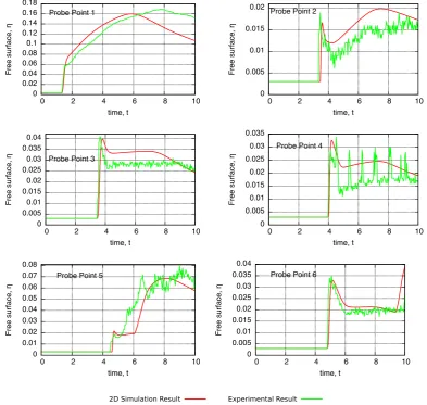
3.11 Final Free Surface Elevation, η after ten seconds. . . 64

3.12 Comparison of the simulation results with the experimental data for the free surface elevation,η after the last time step. The positions of

the probe points are indicated in figure 3.10. . . 65

4.1 Top view of 2D flow domain, Ω2 = Ωc∪Ωf consisting of the river

channel, Ωcand the floodplains, Ωf = Ωf1 ∪Ωf2. . . 70 4.2 Cross sectional view of 2D flow domain, Ω2 _{= Ω}

c∪Ωf consisting of

the river channel, Ωc and the floodplains, Ωf = Ωf1 ∪Ωf2. . . 70 4.3 Channel cross section in HCM without the floodplains, showing the

channel bottom topography, zb(x, y) (in red), the channel wall

ele-vation , zw_b(x), laterally flat free-surface elevation ¯η(x, t), the

bot-tom elevation in 1D sense Zb(x), the top width B(x, zw_b(x)) and

the y−coordinates y_lw(x) := yl(x, zbw(x)) and yrw(x) := yr(x, zwb(x))

respectively of the left and right lateral walls at the channel top.

H(x, y, t) is the depth of water measured fromzb(x, y) to the flat free

surface ¯η(x, t). . . 71

4.4 Top view of Lateral Boundaries (at elevation,z=zw_b (x)) . . . 74

4.5 Diagram explaining the equations solved in the channel. The equa-tions are the 1D Saint Venant model with coupling terms (4.31) and

(4.32) and the lateral discharge equation (4.34). Dotted lines

indi-cate the end of channel region at which the lateral fluxes between the channel and floodplains are computed. . . 77

4.6 Summary of the different models for the different regions of the flow domain. The 1D Saint Venant model with coupling terms, (4.31)

and (4.32) and the lateral discharge equation (4.34) are solved for

the channel flow while the 2D shallow water system (2.32) is solved for the flow in the floodplains. The dotted lines indicate the

bound-aries between the sub domains, the point at which lateral fluxes are

computed and the blue arrows indicate the presence of flow exchange between them. . . 78

4.7 Grid of the entire domain consisting of the 1D grid Ω1D_h at the middle

and the 2D grids Ω2D_h for the floodplains. The grids are matching in the sense that there is no gap between the 1D and the 2D grids. . . 79

4.8 A single cell, Ki in the 1D channel mesh showing its lateral edges;

South edgeeS_i is on the negativey-direction while the North edgeeN_i is on the positivey-direction. These edges are the interfaces between

the 1D cell and the adjacent 2D floodplain cells. . . 80

4.9 To the left is a 1D channel cell and its adjacent 2D floodplain cells while to the right is the 1D cell subdivided into two subcells viewed

4.10 Flow Chart for horizontal Coupling Method depicting the black box

solver and post processing stages. The black box solver stage com-putesWn+1_i ∗using the 1D solver (3.38) and Πn+1_ij , with the 2D solver

(3.30). At the post processing stage, Φn_i is computed with (4.60),

while (qyS/N)n+1_i are computed using (4.46) and (4.47). . . 93

4.11 Comparison of the final free surface elevation for the HCM with those

of the full 2D simulation and the FBM after ten seconds. . . 94

4.12 Comparison of the time evolution of the free surface elevation, η at the probe points indicated in figure 3.10. . . 94

5.1 Cross sectional view of 2D flow domain, Ω2 = Ωc∪Ωf consisting of

the river channel, Ωcand the floodplains, Ωf = Ωf1∪Ωf2. The green curve is the free surface elevation and the red curve is the bottom

topography. . . 97

5.2 Cross section of the channel flow domain without the floodplains in the VCM. It shows the channel bottom topography zb(x, y) (in red),

the channel wall elevation z_bw(x), laterally varying free-surface ele-vation η(x, y, t), the bottom elevation in 1D sense Zb(x), the top

widthB(x, z_bw(x)) and they−coordinatesy_lw(x) andyw_r(x) of the left

and right lateral walls at the channel top. The total water depth H(x, y, t), the channel depth β(x, y), the lower layer water depth

h1(x, y, t) are all measured from the same bottom elevation, zb(x, y).

The upper layer water depth ish2(x, y, t). . . 98

5.3 The two layers in the VCM in the case of full channel (left) and the

non full case (right). . . 104

5.4 Mesh for the two sub-models. . . 114 5.5 Three dimensional view of the channel meshes (without floodplain)

showing a single 1D channel cell,Ki(the largest rectangle in blue) and

the 2D channel cells, Tij (the smaller blue rectangles). The channel

bottom topography is shown in black. The arrows indicate the flow

exchange between the two layers in the channel and it is computed

5.6 Three dimensional view of a single 1D channel cell, Ki (the largest

rectangle in blue), the 2D channel cells, Tij (the smaller blue

rect-angles) and the floodplain mesh (in green). The arrows indicate the

flow exchange between the channel and the floodplain. These

inter-actions are seamlessly computed by the 2D upper layer model while computing the intermediate solutions in the channel. The two layer

model is not solved in the floodplain (green) mesh. . . 115

5.7 Discrete channel geometry in 1D channel cell (figure 5.7(a)) and the cross sectional view of the channel flow 2D channel cells when full

(figure 5.7(b)) and non-full (figure 5.7(c)). . . 116

5.8 Flow chart for the VCM depicting the floodplain flow solver and the channel flow solver. The details of the channel solver is illustrated in

figure 5.9. . . 127

5.9 Details of the channel solver part in the flow chart of the VCM (figure 5.8). It depicts the three-step channel flow solver which implements

the two-layer coupled models, (5.46), (5.47). It also shows the two

stages to solve (step 2) the channel models. Step 2, stage 1 computes the intermediate solutions and the lateral fluxes between the

chan-nel and the floodplains, while step 2, stage 2 enforces the mass and momentum conservation to update each layer solution. . . 128

6.1 Comparison of free surface elevation for the different methods for test

case 1 after the last time step. . . 143 6.2 Comparison of free surface elevation, η at probe points for test case

1. The locations of the probe points are shown in 3.10. . . 144

6.3 Top view of Channel and Floodplain for test case 2 showing the flood-plain region in (x, y)∈[10.5,16.0]×[0,1.8] and the channel region in (x, y)∈[0,19.3]×[1.8,2.3]. . . 145 6.4 Comparison of free surface elevation distribution for the different

methods for test case 2 at the last time step. . . 147

6.5 Comparison of velocity magnitude for the different methods for test

case 2 after the last time step. . . 148 6.6 Comparison of the time variation of the water height at the probe

points for test case 2. . . 149

6.8 Comparison of the time variation of the y-velocity component at

probe the points for test case 2. . . 151 6.9 The bottom topography and the channel wall elevation for test 3 . . 152

6.10 Visualisation of free surface elevation aftert= 40 for test case 3. The

x-axis is from left to right, while they-axis is from the bottom to the top. . . 153

6.11 Visualisation ofx-velocity after t= 40sfor test case 3. Thex-axis is

from left to right, while they-axis is from the bottom to the top . . 154 6.12 Visualisation ofy-velocity aftert= 40sfor test case 3. The x-axis is

from left to right, while they-axis is from the bottom to the top. . . 154

6.13 Visualisation of velocity magnitude after t= 40sfor test case 3. The x-axis is from left to right, while they-axis is from the bottom to the

top . . . 155

6.14 Time variation of water depthH (left column),x-velocity component (middle column) andy-velocity component (right column) at selected

probe points within the channel for test case 3. Each row corresponds

to one probe point which is indicated on they-axis of the water depth H plot on the left. . . 156

6.15 Time variation of water depth H (left column), x-velocity compo-nent (middle column) and y-velocity component (right column) at

the indicated probe points in the floodplain for test case 3. Each row

Acknowledgments

Firstly, I would like to express my sincere gratitude to my supervisor Dr Andreas

Dedner for his continuous support of my Ph.D study. Dr Andreas’ vast knowledge

and expertise were not only source of ideas but have also been great motivation to

me throughout the period. Every meeting with him during the period provided me

with the relevant answers that I needed and initiated great thoughts and reflections

that broadened the scope of this study. His patience, especially during the tough

times in the Ph.D pursuit, is deeply appreciated.

I am grateful to the Petroleum Technology Development Fund (PTDF),

Nige-ria for funding this study. I thank the former President of NigeNige-ria Dr Goodluck

Jonathan who provided Nigerians equal opportunities devoid of godfather-ism, hence

people like me could compete and obtain this prestigious scholarship award.

I also wish to thank the Director of the Center for Scientific Computing,

Prof. Mark Rodger for his kindness towards me before and throughout the period

of my study in Warwick. Prof. Rodger’s support was instrumental for my being a

recipient of the Chancellor’s International Scholarship award, even though I later

turned it down for the PTDF award. I also express my appreciation to all the staff

in Warwick, especially Mrs. Glanville Vida, the CSC secretary who has been more

than supportive. To my follow Ph.D students, I say thanks for the times we shared

together especially during lunch and FATNode dinners.

Special thanks to my family: my wife, my sons, my mother and to my

brothers and sisters for their continuous prayers.

Finally, I return all glory to my heavenly father, the Almighty God for making

Abstract

Abbreviations

• NSE Navier-Stokes Equations.

• FSEE Free Surface Euler Equations.

• SWE Shallow Water Equations.

• SVM Saint Venant Model.

• HRM Hydrostatic Reconstruction Method.

• FBM Flux-Based Method.

• HCM Horizontal Coupling Method.

• VCM Vertical Coupling Method.

List of Symbols

~

X = (x, y)∈_R2_.

z∈_R.

t: Time variable.

η(X~, t): Free surface elevation in 2D.

¯

η(x, t): Laterally averaged free surface.

∂tu: The derivative of u with respect to t.

u=u(X~, z, t) : 3D velocity component along x-direction.

v=v(X~ , z, t) : 3D velocity component along y-direction.

w=w(X~ , z, t) : 3D velocity component alongz-direction.

~

U := (u, v, w)T : The velocity vector in 3D.

~

u:= (u, v)T: 3D Velocity vector with only the xand y components.

∇_3D = (∂x, ∂y, ∂z)T.

∇= (∂x, ∂y)T.

∆3D = (∂xx2 +∂yy2 +∂2zz).

g: Acceleration due to gravity.

H(X~ , t): Water depth in 2D.

H(x, y): Water depth in 1D models.

¯

u(X~ , t): x-component of velocity in 2D.

¯

v(X~, t): y-component of velocity in 2D.

qx(X~ , t): 2D discharge along x-direction.

qy(X~, t): 2D discharge alongy-direction.

zb(x, y): 2D bottom topography.

Zb(x): 1D bottom topograghy.

z_bw(x): Channel wall elevation.

B(x, z): Channel lateral width.

yl(x, z): y-coordinate of channel left wall.

yw

l (x) :=yl(x, zbw(x)): y-coordinate of channel left wall at the top.

yr(x, y): y-coordinate of channel right wall.

A(x, t): Channel cross sectional area.

Q(x, t): Sectionally-averaged discharge.

W = (A, Q)T: Solution vector in 1D channel model.

u(x, t) = Q_A: Sectionally averaged veloicty.

Π = (H, qx, qy)T: Solution vector in 2D SWE.

F1: Flux function alongx-direction.

F2: Flux function alongy-direction.

F = (F1, F2): The 2D flux vector function in the 2D SWE.

H(A, zb): Function that returns height given the wetted cross sectional area and

bottom evelevation.

φ: 1D numerical flux function.

Φ = (ΦA_,ΦQ_{): Coupling term in HCM.}

φ2D: 2D numerical flux function.

Ki: 1D grid cell.

K_iN: Subcell ofKi on the North side.

K_iS: Subcell ofKi on the South side.

(W)N_i ,(W)S_i : 2D solution vectors inK_iN, K_iS respectively.

(Tij)N: 2D cell adjacent to 1D cell Ki on the North side.

(Tij)S: 2D cell adjacent to 1D cell Ki on the South side.

(Π)N_ij,(Π)S_ij: 2D solution vectors in (Tij)N,(Tij)S respectively.

β(X~ ): Channel depth.

Ac(x): Area equal to that of an exacly filled channel.

η1(x, t): Top elevation of lower layer in the VCM.

h1(X~, t): Lower layer water depth in VCM.

A1(x, t): Wetted crossectional area of the lower layer.

Q1(x, t): Sectionally averaged discharge of the lower layer.

u₁ = Q1

A1: Sectionally averaged velocity in the lower layer.

h2(X~, t): Water depth in the upper layer.

~

q2: 2D discharge vector in the upper layer.

Tij: Upper layer 2D channel cell corresponding with the lower layer cell, Ki.

A: Computes the total water area in a channel cross section given the free surface

distribution.

βij: Channel dept in upper layer cellTij.

∆yij: Width of 2D channel cell,Tij.

Sij: Mass exchange between upper layer cell,Tij and the lower layer 1D cell Ki.

S_iQ: Total momentum exchange between the lower layer and all the 2D upper layer

cells,Tij.

A2,i: Sum of all wetted area in the upper layer.

A1,i: Wetted cross sectional area in the lower layer.

Ai=A1,i+A2,i.

~uη1,i,j= (uη1,i,j, vη1,i,j)

T_{: The interface velocity.}

Chapter 1

Introduction

1.1

Introduction

All over the world, flooding is a recurring natural disaster that has led to the loss of over 500,000 human lives [Doocy et al., 2013] and caused the damage of properties

worth over 80 billion dollars [Smith and Katz, 2013]. In most flooding events,

ba-sic facilities such as transportation and communication systems, water and power lines, schools and offices, among others, are usually destroyed while survivors are

temporarily or permanently displaced from their homes. [Doocy et al., 2013]

re-viewed flooding events in the period of 1980 to 2009. Their findings indicate that 539,811 deaths and 361,974 injuries were recorded and 2,821,895,005 people affected

in one way or the other due to flooding within the period under review [Doocy et al.,

2013]. In 2010, several countries and regions, such as Central Europe, North East-ern Brazil, South West of China, etc, were severely hit by flood disasters [Wang,

2011]. In 2012, Nigeria experienced one of the country’s worst flood incidences as several states of the country were devastated by flood [Agbonkhese et al., 2014].

According to the account in [Tawari-Fufeyin et al., 2015], Cameroun experienced

sustained rainfall between June and September, 2012 which caused excessive flood-ing around the Ledja Dam and led to the break of the dam. Hence, water flowed

into Nigerian seas through River Benue, through River Niger, causing eleven states

(about one-third of the country) to be flooded [Tawari-Fufeyin et al., 2015].

Unfortunately, important human activities, like urbanisation and

deforesta-tion, contribute to increased frequency of flooding; in Urbanisadeforesta-tion, impermeable

materials like tarmac and concrete are used for roads, while deforestation involves the reduction of vegetation cover, see [Jackson, 2016]. Both of these prevent rain

may lead to river flooding, see [Jackson, 2016] Climate change is also another factor

that increases the risk of flooding [Pitt, 2007]. Therefore, there does not seem that there is an end in sight to flooding. On the other hand, flooding is advantageous

with regards to improving soil fertility, natural irrigation, propagation and survival

of some species of plants and shrubs, maintenance of the ecosystem, among others [Kharat, 2009].

Consequently, it is environmentally unfriendly and technically not possible

to totally eliminate flooding. Therefore, an effective way of managing flood risks are being established [Kharat, 2009]. Flood risk management is established for this

purpose. The aim is to design comprehensive plan to reduce the possibility and/or

effects of floods, which might include prevention, monitoring, recovery, preparedness and control of flood risk [Wang, 2011].

An important component of flood risk management, as also recommended

in [Pitt, 2007], is the development of techniques and tools for predicting floods [Kharat, 2009; Wang, 2011]. The insights and information gained from such

pre-dicting tools can be used to develop flood maps, carry out development planing,

prepare emergency plans, undertake risk assessment based on susceptibility data for various socio-economic factors, and for learning lessons on sources and courses of

flooding [Kharat, 2009]. The information can also facilitate communication of flood risk among stakeholders such as professionals, politicians, public and other interest

groups [Pender and N´eelz, 2007]. Finally, they can be used for disaster education

and evacuation planning and training.

In order to develop such predicting tools, physical (experimental) models or

mathematical (computer) models can be used [Kharat, 2009; Wang, 2011].

How-ever, flood-type experiments could be costly, time consuming and difficult to be reused in different scenarios. Hence, mathematical-computer models are viable

op-tion [Kharat, 2009]. This thesis, is therefore concerned with developing

compu-tationally efficient computer-based models for simultaneously simulating the flow and flooding of rivers. These methods are what is referred to as coupling methods

throughout this thesis and in the literature also.

The rest of this chapter is organised as follows. In section 1.2, we briefly describe the basis for the derivation of the mathematical equations usually adopted

for flood simulations. We leave the details of the derivations for chapter 2. In section

1.3, we briefly explain the main idea in coupling methods. This is to make the graphics and discussions in the subsequent chapters easy to understand. We state

the specific objectives of the research in section 1.4 and review coupling methods in

1.2

Flood Flow Simulation

Having identified the need for flood simulations using computer-based methods, we

now briefly discuss the approach with which the mathematical equations governing flood flows are derived. We leave the details for a later chapter. As the region

occupied by flood can be large compared to the height of flood, we can consider

flood flows as shallow water flows. This means that the vertical height of the fluid is very small compared to the horizontal length, so the vertical accelerations are

neglected and fluid pressure is taken to be hydrostatic [Stoker, 1957; Toro, 2001;

Aldrighetti, 2007; Decoene et al., 2009]. This leads to the shallow water equations which have been widely accepted for modelling shallow flows such as flood flows,

river flows, tsunamis, etc [Toro, 2001].

Several researchers have used the shallow water equations for flood

simula-tions, see [Mignot et al., 2006; Hunter et al., 2008; Liang, 2010; Wang, 2011] for

examples. However, we are particularly interested in river flooding, that is floods caused by river overflow. River flooding occurs when water enters into the river

causing its discharge to exceed its capacity, hence the river overflows onto the

sur-rounding environments [Jackson, 2016]. These sursur-rounding environments which can be flooded by water from the river, are called the floodplains. River flooding is very

common and rarely absent in any flooding event since they are triggered once too

much water enters into the river. A typical example is the Nigerian incidence of 2012 [Agbonkhese et al., 2014; Tawari-Fufeyin et al., 2015].

To simulate river flooding, it is necessary to simulate both the flow of water

along the river channel and flow of water in the floodplains. Assuming the task is to simulate just the river flow alone, then one could assume that river flow is

dominated along the river course neglecting variations in flow velocities and

free-surface along the vertical and lateral directions, leading to the one-dimensional (1D) St. Venant’s model [Stoker, 1957; Cunge et al., 1980; Decoene et al., 2009]. This 1D

model is computational inexpensive [Blad´e et al., 2012; Morales-Hern´andez et al.,

2013]. However, during flooding when the river overflows, one needs to simulate the flows in both the river and the floodplains. In this case, the 1D model is no

longer valid as the flow, especially in the floodplains, has become multidimensional.

The problem then arises that even a two-dimensional (2D) simulation of flows in both floodplains and channel, is computationally expensive due to more complicated

equations than 1D, data requirements and smaller time steps [Blad´e et al., 2012; Morales-Hern´andez et al., 2013].

whole domain while 2D simulation is computationally expensive. Fortunately, the

1D assumptions could be retained along the river channel [Fernandez-Nieto et al., 2010]; moreover, the 2D floodplains might be small compared to the entire domain.

Therefore, an approach is to decouple the domain, use the 1D model in the river

channel and use the 2D model in the floodplains [Fernandez-Nieto et al., 2010; Blad´e et al., 2012; Morales-Hern´andez et al., 2013; Goutal et al., 2014]. The problem of

efficiently coupling the two sub-models then arises. This has been the subject of

much research, as we review in section 1.5 below, and also the goal of the current research. Therefore, the objective of this thesis is to develop methods to efficiently

couple a 1D river model with a 2D flood model for simulating floods.

1.3

The Main Ideas in Coupling Channel and

Flood-plain Flow Models

In this section, we present some graphics to briefly explain the main idea in coupling channel and floodplain flow models. Imagine the flow of water over a fixed 2D

horizontal domain comprising of a channel and floodplains, see figure 1.1. Figure

Figure 1.1: Shallow water flow over a domain with bottom topographyzb(x, y) (in

1.2 shows a cross section of the flow domain in figure 1.1 at a fixedx. For this cross

section the channel is in the region ya ≤ y ≤yb while the floodplain occupies the

remaining region.

Figure 1.2: Cross section at a fixed pointxin the flow domain depicted in figure 1.1. The bottom topography (in red) comprises of the channel in the regionya≤y≤yb

and the floodplain which occupies the remaining regions. The free surface elevation is in green andH(x, y, t) is the water depth.

The idea of coupling methods is to decouple the cross section in figure 1.2, into the channel region and the floodplain regions. This is illustrated in figure 1.3.

Figure 1.3: Cross section at a fixed x in the flow domain showing the different regions for channel and the floodplains. The middle region is the channel which occupies the regionya≤y≤yb while the left and right regions are the floodplains.

Then, the 2D shallow water flow model is applied to the flow in the

flood-plains, while a channel flow model is used for the flow in the channel region. Figure 1.4 illustrates this idea. Since the standard 1D channel flow model (presented in

chapter 2.4) does not account for the interaction between the flows in the channel

Figure 1.4: A picture of the different models for the different regions. The 2D shallow water equations for the floodplain flow (left and right) and a channel flow model for the channel region (middle).

of coupling methods is to propose models for the channel flow. Different methods propose different models for the channel flow. Therefore, the channel flow model is

what actually defers for different coupling methods. Hence, it is usually necessary

to depict the problem by showing only the channel cross section without the need to include the floodplains, see figure 1.5. Therefore, in all the methods we propose

in this thesis, we depict only the channel flow region. For instance, the horizontal

coupling method (HCM) proposes the standard Saint Venant open channel model including a coupling term and the use of the y-component discharge equation for

the channel flow. This is depicted in 1.6(a). While the vertical coupling method proposes two-layer models for the channel flow, see figure 1.6(b). Details of these

methods are given in subsequent chapters.

The specific objectives of this thesis are listed in the following section.

1.4

Research Objectives

This thesis aims to propose and implement methods to coupled the 2D shallow

water equations with the 1D St Venant open channel model that will allow for the

efficient and accurate simulation of river flooding. It is also intended to validate the methods using some hypothetical test cases. Specifically, this thesis aims to achieve

the following objectives.

• Implement and test a 2D numerical solver for the 2D shallow water flow models using a well-balanced method.

• Implement and test a 1D numerical solver for the 1D St Venant open channel

Figure 1.5: Flow cross section depicting only the channel region (channel cross section). Channel model is derived for the flow in this region. The flow in the flood-plains are used as boundary conditions. The channel flow also serve as boundary conditions for the 2D floodplain models.

(a) Physical structure of the channel flow in the horizontal coupling method. The channel flow is modelled with (i) The Saint Venant Model with coupling term and (ii) the lateral discharge equation in the 2D shallow water equations

(b) Physical structure of the channel flow in the vertical coupling method. The channel flow is described with two-layer models - the upper layer model and lower layer model. The blue line separates the two layers.

• Implement the 2D/1D coupling method proposed in Blad´e et al. [2012],

com-pare the result with full 2D solver, then propose and implement a coupling method following the lines of the mathematical formulations in [Marin and

Monnier, 2009].

• Propose and implement a completely new coupling method based on vertical

partitioning of channel flow.

• Validate all the proposed methods using hypothetical data.

In the following section, a review of some existing coupling methods is presented.

1.5

Review of Coupling Methods

As mentioned above, coupling methods aim to utilise the advantages of the

compu-tational efficiency of the 1D river model and the accuracy of the 2D flood model. Early attempts to couple river and floodplain flows were developed as extension of

existing 1D river models where the floodplain is modelled by using storage areas,

see [Cunge et al., 1980; Blad´e et al., 1994] for example. But this approach does not allow to study the dynamics of flow in the floodplains [Fernandez-Nieto et al., 2010].

Hence, methods which allow to simultaneously simulate the flow dynamics in both

the river and floodplains are being developed.

In [Blad´e et al., 2012], a method for numerically coupling the 1D model and

2D was developed. The authors used the 1D St Venant model for the main river

channel and the 2D shallow water model for floodplain flows. Coupling is then achieved through numerical fluxes in the finite volume discretization of the models.

They called the method, the Flux-Based Method (FBM).

Another idea which uses the theory of characteristics to formulate a 1D and 2D coupling method is presented in [Chen et al., 2012]. In this approach, the 1D and

2D models are the same as those in [Blad´e et al., 2012]. The 1D model was solved

with the implicit four-point Preissmann scheme while the 2D model was solved with a PISO-like algorithm. They considered only boundary-to-boundary (frontal)

coupling. To couple the two models, they defined some matching conditions at

the boundary points. Then a prediction and correction algorithm was designed to ensure that the matching conditions are satisfied. The 1D and 2D shallow water

model each coupled with the sediment transport model was studied in [Zhang et al.,

In another study [Seyoun et al., 2012], the 1D river model was coupled with

the 2D non-inertia model to simulate the interaction of a sewer system with over-land flow. The authors used the 1D model implemented in SWMM5 [Rossman

et al., 2005] which is a finite difference approximation of the 1D shallow water

sys-tem. They solved the 2D model using the alternating direction implicit(ADI) finite difference scheme. The discharges at the 2D/1D interface are calculated according

to the water level differences between the flows in the two domains. This study used

the non-inertia 2D models which ignore the convective terms in the shallow water models.

Two different methods of coupling 1D and 2D models were developed in

[Morales-Hern´andez et al., 2013], see also [Morales-Hern´andez, 2014]. The methods are also based on existing 1D and 2D models. The two models are solved with

explicit finite volume methods. The authors defined what is called the coupling zone

which is an intersection line between the sub-domains. They called the methods the only mass conservation(OMC) and mass momentum conservation (MMC) methods.

Both methods are based on post-processing of separately computed solutions of the

existing 1D and 2D models. For both methods, each model(1D and 2D) computes its own time step and the minimum is chosen as the current time step. For the

OMC method, each model updates its own cell averages independently. The updated values in the 2D and 1D cells at the coupling zone do not account for the interaction

between the two sub-domains. Hence, these updated values are regarded as star solutionsat the coupling zone. With thesestar solutions, the total water volume in a 1D cell and all its adjacent 2D cells is computed from which a common water

level is found for all the cells. Using this common water level, the water height

for 2D cells and the wetted area for the associated 1D cell are found. These are taken as the new cell averages for the new time level. For the MMC approach,

in addition to the above procedure, a similar approach is also adopted to enforce

momentum conservation which then enables to compute the new discharges for all the 1D and 2D cells. The possible issues with these methods are: (i) The

post-processing step, which ensures mass and/or momentum conservation, might

not guarantee the accuracy of the solution since it computes the free-surface to be laterally constant in each 1D cell and its adjacent 2D cells and; (ii) The first step

where the conserved variables were updated to get star values, may give inadequate

results at coupling zone since the calculation completely ignores the interaction between the two sub-domains. Recently, these strategies were applied to Tiber

River, Rome in [Morales-Hern´andez et al., 2016].

authors classically derived the exchange terms in the 1D model from the full 3D

Navier-Stokes equations and numerically coupled the 1D and 2D models using an optimal control process. In [Fernandez-Nieto et al., 2010], the superposition

ap-proach of [Marin and Monnier, 2009] was extended to finite volume methods in

which a discrete exchange term that leads to globally well-balanced scheme, was derived. In this approach, a 2D grid is superposed over the 1D channel grid and a

Schwartz-like iterative algorithm is used to achieve convergence. The challenge in

this method is that in practical cases, the iterative process can jeopardise the overall efficiency of the method [Goutal et al., 2014].

In all the coupling methods, a great difficulty is the calculation of the lateral

discharge along the river channel since the 1D model does not have an equation to compute it. In [Ghostine et al., 2015], the lateral discharge was set to zero and

used in evaluating 2D numerical fluxes at the interfaces between 1D region and 2D

region. Using the models and exchange terms derived in [Marin and Monnier, 2009], a strategy to estimate this lateral discharge without superposition or overlapping,

was proposed in [Goutal et al., 2014]. The approach uses an iterative technique

to estimate the transverse velocity. This iterative technique uses the solution of successive Riemann problem. However, the problem of computing the lateral or

transverse discharge/velocity remains a major challenge.

Different classes of coupling approaches have been applied to solve coupled

continuum mechanics problems. Among them are the closely or fully coupled

meth-ods which at each time step, solve the governing equations simultaneously for all the sub-domains, while iterative coupled methods solve the equations iteratively

until convergence is achieved [Von Estorff and Hagen, 2006; Settari and Walters,

2001]. Most of the methods for river-flood coupling are of the closely coupled type, like those in [Blad´e et al., 2012; Morales-Hern´andez, 2014; Ghostine et al., 2015;

Goutal et al., 2014]. A few examples also exist for iterative type methods, like the

superposition method [Marin and Monnier, 2009; Fernandez-Nieto et al., 2010]. In practical cases of river-flood coupling, iterative process might not converge and can

jeopardise the overall efficiency of the method [Goutal et al., 2014]. Therefore, all

the methods considered in this thesis are of the closely coupled type.

In the context of shallow water equations, [Morales-Hern´andez et al., 2013]

classified coupling methods into two types, namely lateral and frontal coupling.

While lateral coupling refers to methods that couple 1D and 2D models in sub-domains that are connected at the lateral boundaries of the channel; frontal coupling

refers to methods that couple the models when the connecting interface is in direction

in computing the lateral discharge mentioned above.

Lateral coupling methods retain 1D assumptions in the channel- that velocity and free surface are laterally uniform - even during flooding. Hence, these methods

are not able to compute the true 2D flow structure in the channel during flooding.

On the other hand, frontal coupling methods are able to compute 2D flow structure in the channel but they loose efficiency because they compute the 2D solutions at

all times even when flooding seizes to occur. Hence, we need methods that can

compute 2D flow structure in the channel only during flooding and revert back to compute 1D solution when flooding seizes.

In addition to the above limitations, most of the existing methods require

the knowledge of flooding regions a priori. In reality, flooding locations would vary with time, so might be impossible to know a priori. Another issue is that majority of

existing methods are either lateral or frontal type, not being able to automatically

switch types. Finally, methods that are superset of several existing methods are desirable. Hence, it would be important to develop methods that :

1. Compute the 2D flow structure within the channel during flooding but revert

back to 1D simulation if not flooding.

2. Do not require a priori knowledge of the flooding locations but are able to

automatically detect them.

3. Automatically resolve both frontal and lateral type flooding problems without having to use multiple methods.

4. Are superset of existing methods, reducing to different methods under different

choices of model parameters.

In this thesis, two coupling methods are proposed not only for the purpose

of achieving good accuracy and efficiency but also to achieve the goals listed above.

The first one is based on the derivation in [Marin and Monnier, 2009]. In this method, we derive a model similar to the one in [Marin and Monnier, 2009] and

propose to compute the transverse discharge using the third equation of the 2D

shallow water equation. The second method, called the Vertical Coupling Method (VCM), is a completely new approach where the transverse velocity is automatically

computed, flooding regions are automatically detected and it is a superset of different

methods. Well-balanced schemes are schemes that satisfy steady state solutions at discrete level [Greenberg and Leroux, 1996]. A coupling method is said to satisfy the

no-numerical flooding property if it does not erroneously produce flooding when the

for the stability of a coupling method. The methods proposed in this thesis are

shown to be well-balanced and satisfy the no-numerical flooding property.

The scope of this project is to propose these methods, prove their properties,

numerically show their accuracy compared with the FBM, and show that the VCM

computes 2D solutions in the channel only during flooding. Then, we briefly explain (without numerical details) how the VCM is a unifying method. The thesis does not

consider lateral coupling methods. These and other issues are listed as suggestions

for further work.

1.6

Outline of the Thesis

The outline of the thesis is the following. In chapter 2, the 2D shallow water flow model and the 1D St Venant open channel flow model are separately derived for the

case where there is no linking between the two models. The procedure adopted is to

start from the three-dimensional (3D) Navier Stokes equations (NSE), then obtain the 3D free-surface Euler’s equations (FSEE) and finally obtain the 2D SWE. Then

the FSEE is revisited from which the 1D St Venant model (SVM) for open channel

is obtained. A few mathematical properties of these equations are briefly discussed. In chapter 3, an overview of the numerical methods for the models derived in

chapter 2 is presented. Starting from discussing conservative numerical methods, we

introduce the finite volume methods for 1D system of conservation laws. Then we outline one existing finite volume method for the channel flow model and one for the

2D SWE (the flood models). We present a few numerical experiments to verify our

implementation of the methods discussed in the chapter. We also show numerically that the 1D assumption along the channel when not overflowing is valid, justifying

the need for model coupling. Furthermore, we show that the 2D flow structure

within the channel during flooding is not completely absent, motivating the vertical coupling method.

Chapter 4 presents our first coupling method, the HCM. We motivate the

approach by explaining why it is important not to always assume that the channel lateral discharges are zero or even constant during flooding. Following the approach

in [Marin and Monnier, 2009], we revisit the derivation of the SVM in chapter 2

and now assume that the channel is full but still maintaining a laterally flat free surface. This allowed us to derive St Venant model with coupling term. Then we

formulate a finite volume scheme for the model including the discrete coupling term in closed form. We also propose to solve the y-discharge equation in the 2D SWE

flooding and prove that the proposed method satisfies this property and is also

well-balanced. We use the term no-numerical flooding property to mean that a coupling method does not produce artificial (numerical) flood when the channel is not full.

One numerical experiment is then used to access the performance of the method.

More numerical experiments are carried out in chapter 6. All numerical experiments show that the method gives very promising results.

In chapter 5, we propose our new coupling method, the VCM. Unlike the

derivation of the HCM, here we take the channel to be full and that the free surface is not laterally flat. This means that we allow a true 2D flow structure. But we require that the channel free surface be laterally flat when the channel is not

full. This allows us to return to 1D simulations should the channel not be full. The channel is then partitioned vertically into two layers. The lower layer flow is assumed

to be 1D and an appropriate 1D model with exchange term is derived. Similarly, the

upper layer flow is assumed to be 2D and the appropriate 2D model with exchange term is derived. The numerical implementation is then detailed. The numerical

implementation consists of the following three steps. The first step is to distribute

a given 2D solution among the two layers within the channel, the second step is to evolve each layer data using their respective models and compute the lateral flow

exchange between the channel and the floodplains. The third and last step combines the evolved data from the separate layers to evolve the flow to new time level. The

details of these are all presented. The method is proved to be well-balanced and

preserve the no-numerical flooding property.

Chapter 6 presents numerical experiments to access the performance of the

methods proposed in this thesis. We remark that our goal is not for the coupling

methods to reproduce experimental results but to accurately approximate the results of a full 2D simulation. The full 2D model has been widely used to model flooding,

see for example [Mignot et al., 2006; Hunter et al., 2008; Liang, 2010; Wang, 2011],

hence we use it as the reference solution for all the cases considered in this thesis. The results show that the proposed methods are indeed adequate when compared

with the full 2D results. The results also show that the VCM recovers the 2D flow

Chapter 2

Mathematical Models for Flood

and Channel Flows

2.1

Introduction

The general mathematical model governing the flow of a fluid in many applications,

in which the continuum hypothesis is valid, is the Navier-Stokes equations (NSE). Such applications include flows in pipes, seas, oceans, around aircraft and

flood-ing. For a given application, the NSE are complimented with boundary and initial

conditions, which in principle, should enable to completely solve the equations for the problem under investigation. However, for free-surface flows such as flood and

channel flows, amongst many others, the position of the boundary of the flow

do-main is usually not known a priori. This makes a direct application of the NSE to free-surface flow problems difficult as the boundary conditions can not be directly

specified. In addition to the above difficulty, solving the full 3D NSE is

computa-tionally expensive as there does not exist an exact analytical solution for the general 3D NSE. Therefore, to solve a free-surface flow problem, further model derivation is

usually carried out, with the hope of simplifying the NSE into less computationally

expensive models and also to circumvent the unknown boundary position problem. For some flows, like those in seas, rivers, floods, atmosphere, and open

chan-nels, amongst many others, the horizontal length scales (like river length) are much larger than the vertical length scales, like fluid depth [Stoker, 1957; de Boer, 2003].

This allows to assume that vertical component of acceleration is negligible, which in

turn, leads to the assumption of hydrostatic pressure distribution, which means that the net pressure exerted on a fluid particle is only due to the force exerted on it by

With the above approximation, the shallow water theory is established where the

unknown free-surface position, η(X~ , t) is formulated as part of the solution of the problem. The aim of this chapter is to derive the 2D Shallow Water Equations

and the 1D Saint Venant Model needed to simulate flood and open channel flows

respectively, in the following chapters. The chapter also provides the foundation for all the derivations in the following chapters.

The rest of this chapter is organised as follows. Starting with the NSE, the 3D

free-surface Eulers Equations (FSEE) is derived in section 2.2, then the 2D shallow water equations (SWE) is derived in section 2.3. Section 2.4 presents the derivation

of the 1D Saint Venant Model (SVM) for open channel with arbitrary shaped

geom-etry, from which the special SVM for a locally rectangular cross-sectional channel, and also the constant width 1D SWE are obtained. Then the chapter is concluded in

section 2.5 where it is briefly shown that the models derived in the previous sections

are hyperbolic conservation laws with source terms, also referred to as balance laws. Some important properties of such partial differential equations that necessitate

their types of methods of solution, are also briefly outlined.

2.2

The Free-Surface Euler Equations

While the NSE is the model for general fluid problems, the free-surface Euler

equa-tions (FSEE) is the model which govern the flow of an incompressible, inviscid flow under gravity. In this section, we derive the FSEE from the incompressible NSE.

2.2.1 Background

Consider the flow of an incompressible fluid which at time, toccupies the domain, Ωt defined by

Ωt={(X~ , z)∈R3 :X~ = (x, y)∈ΩH ⊂R2 fixed,zb(X~ )≤z≤η(X~ , t)}. (2.1)

The domain is bounded below by a fixed bottom, zb(X~) and above by the

free-surface position,η(X~, t) given by

η(X~ , t) =zb(X~) +H(X~ , t). (2.2)

whereH(X~ , t) is the depth of fluid at time, t, see figure 2.1.

Figure 2.1: Shallow water flow over a domain with bottom topographyzb(x, y) (in

red). The water depth is H(x, y, t) and the free surface elevation is η(x, y, t) (in green). Symboltis time variable and (x, y, z)∈_R3_.

Navier-Stokes Equations (NSE), namely

∇_3D·U~ = 0. (2.3)

∂tU~ +

~

U· ∇_3DU~ =−1

ρ∇3DP+ν∆3DU~ +~g. (2.4)

where U~ = U~(X~ , z, t) = u(X~ , z, t), v(X~ , z, t), w(X~ , z, t)T and P = P(X~, z, t)

are the fluid velocity and pressure respectively at the point (X~, z) ∈ Ωt at time,

t. While ν and ρ are the fluid viscosity coefficient and fluid density respectively and ~g = (0,0,−g)T, where g is the constant acceleration due to gravity. ∇_3D = (∂x, ∂y, ∂z)T and ∆3D = (∂xx2 +∂yy2 +∂2zz).

2.2.2 Deriving the free-surface Euler Equations

To derive the FSEE, the following assumptions are made [Lannes, 2013].

i The fluid is homogeneous and inviscid.

ii The fluid particles do not cross the bottom and the free-surface.

The first assumption means that the NSE, (2.3)-(2.4) reduce to the inviscid

Euler Equations (2.5)-(2.6) below, while the second assumption implies that the kinematic boundary condition holds on both the bottom and free-surface, namely

equations (2.7) and (2.8) respectively. And the last assumption gives rise to the

dynamic boundary condition on the free-surface, namely equation (2.9).

∇_3D·U~ = 0. (2.5)

∂tU~ +

~

U· ∇_3DU~ =−1

ρ∇3DP +~g. (2.6)

(u~ · ∇)zb(X~)−w(X~ , z, t)

z=zb(X~)

= 0. (2.7)

∂tη(X~, t) + (u~ · ∇)η(X~ , t)−w(X~ , z, t)

z=η(X~,t)

= 0. (2.8)

P(X~ , z, t) =Patm on z=η(X~ , t). (2.9)

Here,~u= (u(X~ , z, t), v(X~ , z, t))T_{,∇= (∂}

x, ∂y)T and Patm is the atmospheric

pres-sure, which is usually conveniently taken to be zero. We take it to be zero throughout

this thesis. In the remainder of this thesis, we shall drop the notations for dependent variables on the 3D velocity components. This is for convenience and to allow for

easy read.

Equations (2.5) - (2.9) are known as the Free-Surface Euler Equations (FSEE) [Lannes, 2013]. These are the fundamental equations from which all the models

needed in this thesis shall be derived. To derive the models in the subsequent

chapters, the continuity and momentum equations (2.5)-(2.6) shall be integrated component by component. For this reason, we also write the FSEE, (2.5) - (2.9), in

component form, namely

∇3D·U~ = 0. (2.10)

∂tu+U~ ·(∇3Du) =−

1

ρ∂xP. (2.11)

∂tv+U~ ·(∇3Dv) =−

1

ρ∂yP. (2.12)

∂tw+U~ ·(∇3Dw) =−

1

ρ∂zP−g. (2.13)

~

u·(∇z_b(X~ ))−w

z=zb(X~)

∂tη(X~ , t) +~u·(∇η(X~ , t))−w

z=η(X~,t)

= 0. (2.15)

P(X~ , z, t) =Patm on z=η(X~ , t). (2.16)

2.3

Derivation of 2D Shallow Water Equations

As stated in the introductory section of this chapter, the shallow water theory,

commonly referred to as the theory of long waves [Stoker, 1957], assumes that the depth of water is significantly small compared to horizontal length scales such as

wave length [Toro, 2001; Lannes, 2013; Stoker, 1957; Tanguy, 2010]. In this section,

starting from the FSEE (2.10)-(2.16), we shall derive the Shallow Water equations (SWE), along the lines followed in [Toro, 2001; Tanguy, 2010]. The assumption of

small depth in comparison with horizontal length scales, allows to assume that the

vertical component of acceleration is negligible, that is

d dtw(

~

X, z, t) :=∂tw+U~ ·(∇3Dw) = 0. (2.17)

where we have dropped the independent variable notations for convenience. This

means that the left hand side of equation (2.13) in FSEE vanishes, reducing it to the following equation:

−1

ρ∂zP(X~ , z, t) =g. (2.18)

Integrating equation (2.18) with respect tozand using the dynamic boundary condition (2.16), the pressure is obtained as

P(X~ , z, t) =ρg(η(X~ , t)−z). (2.19)

Equation (2.19) defines the pressure as being hydrostatic which means that the pressure depends only on gravity. Differentiating equation (2.19) with respect tox

andy gives

∂xP(X~ , z, t) =ρg∂xη(X~, t), ∂yP(X~ , z, t) =ρg∂yη(X~, t). (2.20)

The FSEE (2.10)-(2.16) then reduce to the following:

∇3D ·U~ = 0. (2.21)

∂tu+∇3D ·(u ~U) =−g∂xη(X~ , t). (2.22)

together with the kinematic boundary conditions (2.14) and (2.15). We have used

the the vector identity,

∇_3D·(u ~U) =u(∇_3D·U~) +U~ ·(∇_3Du)

and the continuity equation (2.10) to put the left hand sides of (2.22) and (2.23) in

conservative forms.

Notice that the right hand sides of (2.22) and (2.23) are independent of z,

hence their left hand sides being the total derivatives,du/dt and dv/dtrespectively,

are also independent ofz. This means thatuand vare also independent ofz[Stoker, 1957; Toro, 2001]. From this we can conclude that u, v are not very different from

their vertically averaged values, ¯u(X~ , t) and ¯v(X~, t), so we can decompose them into the sum of their averages and some small perturbations, namely

u(X~, z, t) = ¯u(X~ , t) +u_e(X~ , z, t). (2.24)

v(X~ , z, t) = ¯v(X~ , t) +_ev(X~ , z, t). (2.25)

where ˜u(X~, z, t) and ˜v(X~, z, t) are very small perturbations whose average, sum and higher order terms vanish.

Define the discharges alongx and y directions respectively, namely

qx(X~, t) = η(X~,t)

Z

zb(X~)

u(X~ , z, t)dz, (2.26)

qy(X~ , t) = η(X~,t)

Z

zb(X~)

v(X~ , z, t)dz. (2.27)

Integrating the continuity equation (2.21), vertically (over zb(X~ ) ≤ z ≤ η(X~ , t)),

gives

η(X~,t)

Z

zb(X~)

(∂xu+∂yv+∂yw)dz= 0.

Using the Leibniz rule leads to the following equation:

0 =∂x η(X~,t)

Z

zb(X~)

u dz+∂y η(X~,t)

Z

zb(X~)

v dz+

w−~u·(∇η)

z=η

+

~

u·(∇z_b)−w

z=zb

We use the definitions of the averages in equations (2.26) and (2.27) to simplify

the first two terms on the right hand side. Then, use of the kinematic boundary conditions (equations (2.14) and (2.15)) simplifies the last two terms on the right

hand side, hence we have the following equation:

∂xqx(X~ , t) +∂yqy(X~ , t) =−∂tη(X~ , t) =−∂tH(X~ , t). (2.28)

Hence, the following equation, for the depth of water, is obtained:

∂tH(X~ , t) +∂xqx(X~ , t) +∂yqy(X~ , t) = 0. (2.29)

Similarly, if we integrate the x-momentum equation, (2.22) vertically over

zb(X~ )≤z≤η(X~ , t), apply the Leibniz rule, use the kinematic boundary conditions,

(2.14) and (2.15) and the definitions (2.24)-(2.27), then the following equation is obtained:

∂tqx(X~ , t) +∂x

q_x2(X~, t)

H(X~, t)

!

+∂y

qx(X~ , t)qy(X~ , t)

H(X~, t)

!

=−gH(X~, t)∂xη(X~, t)

=−∂x

g

2H

2_{(X~ , t)−gH(X~ , t)∂}

xzb(X~ ).

(2.30)

Finally, if we integrate the y-momentum equation, (2.23) vertically over zb(X~ ) ≤

z≤η(X~ , t), apply the Leibniz rule, use the kinematic boundary conditions, (2.14) and (2.15) and the definitions, (2.24)-(2.27) then the following equation is obtained:

∂tqy(X~ , t) +∂x

qx(X~ , t)qy(X~ , t)

H(X~ , t)

!

+∂y

q_y2(X~ , t)

H(X~ , t)

!

=−gH(X~, t)∂yη(X~ , t)

=−∂_yg 2H

2_{(X~ , t)−gH(X~, t)∂}

yzb(X~ ).

(2.31)

follows:

∂tΠ +∇ ·F(Π) =S(Π, zb),

where Π =

   H qx qy  

, S(Π, zb) = 

 

0 −gH∂_xzb(X~ )

−gH∂yzb(X~)



 ,

F(Π) = (F1(Π), F2(Π)), F1(Π) =

   qx q2 x H + 1 2gH2 qxqy

H





, F2(Π) = 

  

qy qxqy

H q2 y H + 1 2gH 2     . (2.32)

The vertically averaged velocity components along thexandydirections are ¯u(X~ , t) =

qx(X~,t)

H(X~,t) and ¯v(X~ , t) = qy(X~,t)

H(X~,t) respectively.

2.4

1D Saint Venant Equations for an Open Channel

With Varying Width

For flows in rivers and open channels, it can be taken that the flow is dominated

along the longitudinal direction, with negligible velocity and free surface variations along lateral and vertical directions [de Boer, 2003]. This important assumption

enables the derivation of a more simplified model for such flows. In this section,

we derive the set of partial differential equations (PDEs) suitable for dealing with flows in rivers and open channels with arbitrary shaped geometry. These equations,

referred to as the Saint Venant Equations or Saint Venant Models (SVM) were first

derived in [de Saint-Venant, 1871].

The hypothesis of the SVM include those of the FSEE in section 2.2, in

addition to the following :

• The flow is well approximated by a flow with uniform velocity over each

cross-section and the free surface is assumed horizontal over each cross cross-section, namely

η(X~ , t) = ¯η(x, t). (2.33)

• The shallow water assumption in section 2.3 is valid, that is the depth of water is significantly small compared to longitudinal length scales.

We first remark the following: We shall not include friction modelling in the

deriva-tions throughout this thesis but shall use the results from literature like those from

2.4.1 Background

There are different approaches to derive these models, such as (i) the infinitesimal

elemental control volume approach [Stoker, 1957; de Boer, 2003; Tanguy, 2010;

Cunge et al., 1980], (ii) the asymptotic expansion approach [Decoene et al., 2009] and (iii) the direct integration approach [Fernandez-Nieto et al., 2010; Aldrighetti, 2007;

Szymkiewicz, 2010]. Here, and throughout this thesis, we shall consistently adopt

the direct integration approach whereby we directly integrate the FSEE equations.

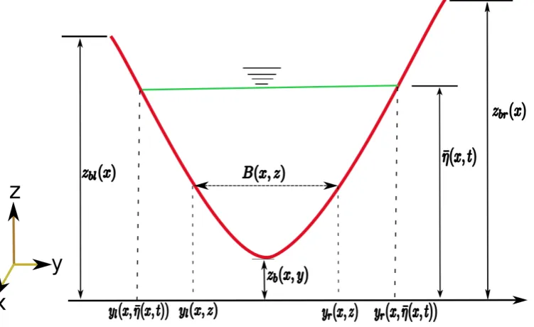
Figure 2.2: Non-full channel flow cross section showing the left and right bank elevationszbl(x) andzbr(x), the laterally flat free-surface elevation ¯η(x, t) (in green),

the bottom elevation in 2D zb(X~ ) (in red), the width, B(x, z) of the channel at

elevation,zabove the reference elevationz= 0, and they−coordinates,yl(x, z) and

yr(x, z) of the left and right lateral walls at elevation z.

We begin by considering an open channel whose length lies along thex-axis

(frontal direction), the width lies along they-axis (lateral direction) and z-axis is in

vertical direction. Figure 2.2 shows a cross section of the channel at pointx along its length. We assume that the complete geometry of the channel is known, so the

bed elevation,zb(x, y) is known at all points. The left and right wall/bank elevation,

zbl(x) andzbr(x) of the channel are also given. Zb(x) is the bottom elevation of the

cross section in 1D sense. Here, we take it to be

Zb(x) = min

At any elevation,zabove the referencez= 0, we define the function,B(x, z) to give

the lateral width of the channel cross section. Furthermore, we define the functions, yl(x, z) andyr(x, z) to give they−coordinates of the left and right lateral boundaries

respectively at elevation,z so that

B(x, z) =yr(x, z)−yl(x, z). (2.34)

Note that the width functions;B(x, z), yl(x, z), yr(x, z) satisfy the following

B(x, z) = 0, yr(x, z) =yl(x, z) for all z < Zb(x). (2.35)

Now, a very important quantity throughout this thesis, is the maximum

channel wall or bank elevation.

Definition 2.4.1(Maximum channel wall elevation,z_bw(x)). The maximum channel wall elevation at cross section x, is the minimum elevation of the channel banks above

which flooding is said to have occurred. We denote it byzw_b (x), that is

z_bw(x) = min(zbl(x), zbr(x)). (2.36)

See Figure 2.2.

We shall use the terms maximum channel wall elevation and channel wall

elevation interchangeably to refer to z_bw(x). Note that this quantity is known since the elevation of both banks are already known. In fact, for the cross section depicted

in Figure 2.2,z_bw(x) =zbl(x).

With the channel geometry completely defined, let ¯η(x, t) be the laterally constant free-surface elevation of fluid in the cross section, see Figure 2.2. Then the

water depth in the cross section is given by

H(X~ , t) = ¯η(x, t)−zb(X~ ), for all yl(x,η¯(x, t))≤y≤yr(x,η¯(x, t)). (2.37)

and the channel flow domain, Ωct at time, t is given by

Ωct={(X~ , z) :yl(x,η¯(x, t))≤y≤yr(x,η¯(x, t)), zb(X~ )≤z≤η¯(x, t))}. (2.38)

Note that the following condition always holds:

zb(X~ )|y=yl(x,z),yr(x,z) =z ∀z∈[Zb(x), z

w

b (x)]. (2.39)