University of Warwick institutional repository: http://go.warwick.ac.uk/wrap
A Thesis Submitted for the Degree of PhD at the University of Warwick
http://go.warwick.ac.uk/wrap/56873
This thesis is made available online and is protected by original copyright. Please scroll down to view the document itself.
JHG 05/2011
Library Declaration and Deposit Agreement
1. STUDENT DETAILS
Please complete the following:
F
2. THESIS DEPOSIT
2.1 I understand that under my registration at the University, I am required to deposit my thesis with the University in BOTH hard copy and in digital format. The digital version should normally be saved as a single pdf file.
2.2 The hard copy will be housed in the University Library. The digital version will be deposited in the (WRAP). Unless otherwise indicated (see 2.3 below) this will be made openly accessible on the Internet and will be supplied to the British Library to be made available online via its Electronic Theses Online Service (EThOS) service.
[At present, the are
not being deposited in WRAP and not being made available via EthOS. This may change in future.]
2.3 In exceptional circumstances, the Chair of the Board of Graduate Studies may grant permission for an embargo to be placed on public access to the hard copy thesis for a limited period. It is also possible to apply separately for an embargo on the digital version. (Further information is available in the Guide to Examinations for Higher Degrees by Research.)
2.4
For all other research degrees, please complete both sections (a) and (b) below:
(a) Hard Copy
I hereby deposit a hard copy of my thesis in the University Library to be made publicly available to readers (please delete as appropriate) EITHER immediately OR after an embargo period of
... months/years as agreed by the Chair of the Board of Graduate Studies.
I agree that my thesis may be photocopied. YES / NO (Please delete as appropriate)
(b) Digital Copy
I hereby deposit a digital copy of my thesis to be held in WRAP and made available via EThOS.
Please choose one of the following options:
EITHER My thesis can be made publicly available online. YES / NO(Please delete as appropriate)
OR My thesis can be made publicly available only after date] (Please give date)
YES / NO(Please delete as appropriate)
OR My full thesis cannot be made publicly available online but I am submitting a separately identified additional, abridged version that can be made available online.
YES / NO (Please delete as appropriate)
OR My thesis cannot be made publicly available online. YES / NO(Please delete as appropriate) Amar Suresh Parmar
Numerical identification of fast structural growth
in stratified turbulence
by
Amar S Parmar
Thesis
Submitted to The University of Warwick
for the degree of
Doctor of Philosophy
Mathematics Institute
Table of Contents
Acknowledgements ix
Declaration x
Abstract xi
Notation and Parameters xii
1 Introduction 1
1.1 Kolmogorov 1941 . . . 3
1.2 Atmospheric Energy Spectrum . . . 4
1.3 Numerical Weather Prediction Models . . . 7
1.4 Main Results of Thesis . . . 8
1.5 Thesis Structure . . . 9
2 Governing Equations 11 2.1 Boussinesq Approximation . . . 11
2.2 Atmospheric Equations . . . 13
3 The Zigzag Instability 16 4 Numerics 20 4.1 Numerical Scheme . . . 20
TABLE OF CONTENTS iii
4.3 Reproduction of Previous Results . . . 22
4.4 Proposal for More Unstable Initial Profiles . . . 28
4.5 Most Unstable Initial Condition . . . 42
4.5.1 Evolution of Vortex Columns and Growth . . . 43
4.5.2 Production of Enstrophy . . . 45
4.5.3 Energies: Transfer and Spectra . . . 64
4.6 Chapter Summary . . . 72
5 Conclusion 74 5.1 Further Work . . . 76
List of Figures
1.1 Variance power spectra of wind and potential temperature near the tropopause from GASP aircraft data. Reproduced from Nastrom and Gage [1, Fig. 3]. . . 6 3.1 Growth of the zigzag instability, frontal views taken at 7, 36 and 75
seconds. Reproduced from Billant and Chomaz (2000, [2]) . . . 18 4.1 Vorticity isosurfaces of simulation with F r = 0.66 and Re = 1060.
Red and blue contours are 60% of vertically averaged maximum ver-tical vorticity. Reproduced from Deloncle et al. [3, Fig. 1, pp.231] . . 22 4.2 Evolution of the pair of vortex columns which began with a sinusoidal
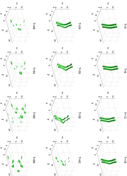
perturbation applied perpendicular to the direction of propagation. . 24 4.3 Evolution of the pair of vortex columns, in they−z plane, with the
initial sinusoidal perturbation applied. . . 25 4.4 Enstrophy evolutions of run F r = 0.66, Re= 1060. Total enstrophy
Z (solid line), horizontal enstrophy Zh (dashed line). Reproduced
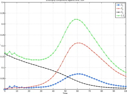
from Deloncle et al. [3, Fig. 2(b), pp.232] . . . 27 4.5 Change through time of the three components of enstrophy and their
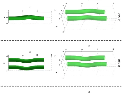
sum for the initial profile with the sinusoidal perturbation. . . 28 4.6 Views of the four different new initial conditions proposed to be more
LIST OF FIGURES v 4.7 Evolution of the pair of vortex columns which began with an offset
perturbation parallel to the direction of travel. The red and blue surfaces are areas of positive and negative potential vorticity. The
P V isosurface thresholds are, in red 0.55·maxx∈D(P V) and in blue
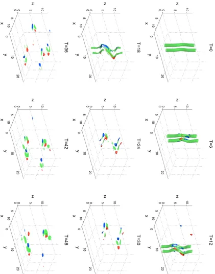
the negative of the same value. . . 33 4.8 Evolution of the pair of vortex columns which began with a coplanar
perturbation perpendicular to the direction of travel. Red and blue surfaces of P V defined as in Fig. 4.7. . . 34 4.9 Evolution of the pair of vortex columns which began with an offset
perturbation in the direction of travel. Red and blue surfaces of P V
defined as in Fig. 4.7. . . 35 4.10 Evolution of the pair of vortex columns which began with a coplanar
perturbation in the direction of travel. Red and blue surfaces of P V
defined as in Fig. 4.7. . . 36 4.11 Evolution of the pair of vortex columns, in the y −z plane, with
the perturbation applied offset in the direction of travel. Enstrophy isosurface value taken as 0.5·maxx∈D(Z). . . 37
4.12 Evolution of the pair of vortex columns, in the y −z plane, with the perturbation applied coplanar perpendicular to the direction of travel. Enstrophy isosurface value taken as 0.5·maxx∈D (Z). . . 38
4.13 Evolution of the pair of vortex columns, in the y−z plane, with the perturbation applied offset perpendicular to the direction of travel. Enstrophy isosurface value taken as 0.5·maxx∈D(Z). . . 39
4.14 Evolution of the pair of vortex columns, in the y−z plane, with the perturbation applied coplanar in the direction of travel. Enstrophy isosurface value taken as 0.5·maxx∈D(Z). . . 40
LIST OF FIGURES vi 4.16 Growth of the zigzag instability measured by furthest distance away
from vortex core. . . 44 4.17 Depictions of the enstrophy profiles of the initial vortex columns. The
core radii, r= 1.315, the separation of the two cores, a= 2.338, and the vortex circulations are Γ1,2 =±10.055. . . 45
4.18 Early time evolution of the pair of vortex columns which began with an offset perturbation parallel to the direction of travel. Red and blue isosurfaces of positive and negative potential vorticity, ±0.55·
maxx∈D(P V). Images shown more frequently than in Fig. 4.7. . . 46
4.19 Early time evolution of the pair of vortex columns, in the y−z plane, with the perturbation applied offset in the direction of travel. Images shown more frequently than in Fig. 4.11. Enstrophy isosurface value taken as 0.5·maxx∈D(Z). . . 47
4.20 Isosurfaces of enstrophy, and enstrophy production through vortex stretching (cyan) and baroclinic production (magenta). Isovalues are; for enstrophy, 0.5 ·maxx∈D(Z); for vortex stretching, 0.8 and for
baroclinic production, 1. . . 50 4.21 Three frames showing isosurfaces of vortex stretching (cyan),
baro-clinic production (magenta) and the total enstrophy production (black) at three different times. Isovalues are; for enstrophy, 0.5·maxx∈D(Z);
for vortex stretching, 0.8; for baroclinic production, 1 and for total enstrophy production, 2. . . 51 4.22 Three frames showing isosurfaces of vortex stretching (cyan),
baro-clinic production (magenta) and the total enstrophy production (black) at three different times. Isovalues for surfaces as in Fig. 4.21. . . 52 4.23 Enstrophy isosurfaces with vortex stretching vectors above the values
LIST OF FIGURES vii 4.24 Enstrophy isosurfaces with vortex stretching vectors at t = 20, a
zoomed in section. . . 54 4.25 Enstrophy isosurfaces with baroclinic production vectors above the
values given in the legends. . . 56 4.26 Enstrophy isosurfaces with baroclinic production vectors att = 14, a
zoomed in section. . . 57 4.27 For t = 2, y−x planes at 6 different z values of vortex stretching
vectors (blue), baroclinic production vectors (red) and the sum of the two. . . 58 4.28 For t = 8, y−x planes at 6 different z values of vortex stretching
vectors (blue), baroclinic production vectors (red) and the sum of the two. . . 59 4.29 For t = 14, y−x planes at 6 different z values of vortex stretching
vectors (blue), baroclinic production vectors (red) and the sum of the two. . . 60 4.30 For t = 20, y−x planes at 6 different z values of vortex stretching
vectors (blue), baroclinic production vectors (red) and the sum of the two. . . 61 4.31 For t = 30, y−x planes at 6 different z values of vortex stretching
vectors (blue), baroclinic production vectors (red) and the sum of the two. . . 62 4.32 For t = 40, y−x planes at 6 different z values of vortex stretching
vectors (blue), baroclinic production vectors (red) and the sum of the two. . . 63 4.33 For t= 20,y−xplanes atz = 4.5 values of vortex stretching vectors
LIST OF FIGURES viii 4.34 Isosurfaces of enstrophy, gradient of temperature, and potential
vor-ticity. Isovalues are; for enstrophy, 0.5·maxx∈D(Z); for∇θ, 0.5 and
for P V ±0.3. . . 65 4.35 Change of x, y and z components of velocity and scalar squared
through time. . . 66 4.36 Evolution of total kinetic energy, total potential energy, scalar
vari-ance dissipation and sum total enstrophy against time. . . 67 4.37 Spectral kinetic energy transfer againsty wavenumber at various times. 69 4.38 Spectral potential energy transfer against y wavenumber at various
times. . . 70 4.39 Kinetic and potential energy spectra againstywavenumber at various
Acknowledgements
I would like to thank my supervisor, Prof. Robert Kerr, for his support, guidance and patience he has shown me during my time studying at Warwick University. I would also like to thank Colm Connaughton and Sergey Nazarenko for their interesting discussions over coffee.
A final thank you to the great friends I’ve made at Warwick and my family for their support and understanding.
Declaration
I wish to declare that this is my own work unless stated otherwise. I state that this thesis has not been submitted for a degree at another university.
Abstract
We investigate a type of instability observed in the presence of two counter rotating vortex
columns in a highly stratified fluid, F r < 1. This instability causes the vortex columns
to be bent and stretched out in the horizontal direction eventually leading to discrete
horizontal layers of vorticity. The instability is known as the zigzag instability and causes
exponential growth in total enstrophy which stops once viscous dissipation becomes
im-portant. We find that two counter rotating vortex columns with localised perturbations
applied parallel to the direction of propagation and offset from one another between the
two columns is an initial profile that is highly unstable to the zigzag instability leading
to exponential enstrophy growth faster than any prior numerical simulations have shown
however is consistent in timing with a previous experimental result. We show that the
zigzag instability that develops on these vortex columns provides a mechanism for energy
(kinetic and potential) to cascade from large scales to small scales.
Notation and Parameters
Name Notation Froude Number F r
Richardson Number Ri
Reynolds Number Re
Brunt V¨ais¨al¨a Frequency N
Density ρ
Gravitational Force gzˆ Pressure p
Velocity u
Vorticity ζ
Viscosity ν
Diffusivity κ
Potential Temperature θ
Strain S
Thermal Expansion Coefficient α
Potential Vorticity ζ · ∇θ
Potential Energy 12θ2
Kinetic Energy 12u2
Enstrophy Z
Vortex Stretching ζSζ
Baroclinic Term αgzζˆ × ∇θ
Chapter 1
Introduction
The nature of turbulent flow means it can potentially act on a huge range of scales, from the very small, through the medium scales that influence the human environ-ment to the vast length scales of planets, solar systems and galaxies. These turbulent flows exist in even the simplest of everyday occurrences, such as the water passing down a plug hole, the movement of air behind a travelling aeroplane and perhaps one of the most important aspects of daily human life, the weather. The on set of turbulence is a complex topic, not least because its characteristics are often defined by a variety of parameters. As an example, the turbulent structures in the Earth’s atmosphere develop and evolve from influences such as the rotation of the planet, heating of the upper layer of the atmosphere by our sun, heating from the surface of the Earth itself, the radius of Earth, its gravitational strength and the fact that that horizontal length scale of the atmosphere is many times greater than the vertical length scale. These though are yet only a few examples of the possible factors that shape the turbulence of Earth’s atmosphere. However, they are more than sufficient to realise immediately that the turbulent structures in the atmosphere of Earth will not be precisely the same on any other of our solar systems planets and perhaps even our galaxies.
1. Introduction 2 da Vinci in the 15th century that first made record of the various structures and
formations within a turbulent flow. The study of turbulence through the use of mathematics was made possible after the development of calculus in the 17thcentury
independently by Newton and Leibnitz which Euler (1757) used to derive an equation for fluid motion based on the principle of momentum conservation
∂u
∂t + (u· ∇)u=
−1
ρ ∇p (1.1)
Though Euler’s equation is certainly of mathematical interest, physically its inter-pretation of fluid motion is limited. One of its primary flaws is the lack of modelling of the interaction between particles which converts kinetic energy to dissipated heat. Euler’s model was improved upon, to take account of energy transitions, by Navier and Stokes independently to give the famous Navier-Stokes equation
∂u
∂t + (u· ∇)u =
−1
ρ ∇p+ν∇
2u+f (1.2)
Coupled with this Navier-Stokes equation, the assumption that the fluid is incom-pressible,
∇ ·u= 0 (1.3) give the fundamental equations that, to this day, many fluid dynamicists study. The addition of the term related to viscosity, ν∇2u, gives rise to the most significant
1. Introduction 3 term, Kolomogorov (1941) was able to show one of the few analytical results of the Navier-Stokes equations relating to energy dissipation.
1.1
Kolmogorov 1941
Turbulent flow involves various scales of motion; large scales that are usually deter-mined by forces and boundaries and small scale motions that obtain their energy from the larger scales. The flow of energy from large scales to small scales proceeds as large scale structures break down into smaller scales which then intern break up to give even smaller scale structures. This process of energy transfer and structure break down continues until the structures become so small that the viscous effects of the fluid dominate over the motion of the structure and then all their energy is dissipated through viscous diffusion.
We define these organised motions of the fluid as eddies. Let the velocity field of a fluid with these so called eddies be defined by the Fourier series [4]
u(x) =Xu˜(k)eikx
and where u˜(k) can be associated with eddies of the size k−1. If we consider a
homogeneous flow which has energy spectrum E(k), and a dissipation spectrum given by 2Re−1k2E(k) then for large Reynolds number, Re, k must also be large for the dissipation spectrum to be significant. Then, the question is, what happens in the range between when the energy spectrum is significant and when the dis-sipation spectrum is significant? Assuming that max (E(k)) occurs when k = k1
and max (2Re−1k2E(k)) occurs when k =k
2 (clearly k1 k2) we call the range of
wavenumbers between k1 and k2 the inertial range[4]. It seems conceivable that in
1. Introduction 4 true, then we could postulate that the energy, E(k), in this range would depend on the wavenumber, k, and the rate per unit at which energy is being transported through the inertial range, ε. That is [5]
E(k)∝εβkγ
Mathematically, we defineεas the averaged sum of squared quantities (henceε≥0),
ε=ν
∂ui
∂xj
+∂uj
∂xi
∂ui
∂xj
+ ∂uj
∂xi
using the standard Einstein summation convention. Dimensionally, the units of;
E(k) is LT32, ε is
U2
T or equivalently
L2
T3 and k is
1
L. Then, dimensionally analysis
yields the only possible solution for β and γ as,
β = 2
3 , γ = 2β−3 =
−5 3 so finally, we have
E(k) =Cε2/3k−5/3 (1.4) for some constant, C.
1.2
Atmospheric Energy Spectrum
struc-1. Introduction 5 tures transferring energy into the large scale structures by amalgamating themselves into these larger structures, this form of energy cascade is typical of 2D turbulence. Regarding the atmosphere, it would seem that the conclusions based on 2D tur-bulence would hold since the vertical length scale of the atmosphere is much less than that of the horizontal length scale, and thus an inverse energy cascade would be expected. However, this has been shown not to be the case and in fact the en-ergy cascade is a forward one as predicted by fully developed 3D turbulence. This is somewhat puzzling, the physical relationship between the vertical and horizon-tal length scales in the atmosphere do not support the idea of fully developed 3D turbulence but nor does the energy spectrum support the idea of 2D turbulence. Perhaps a mechanism exists to transfer energy downscale similar in concept to 3D turbulence but different in its mechanism?
The Kolmogorov prediction of the energy spectrum, (1.4) - k−5/3, is something that has been observed experimentally in the atmosphere. In 1985 Nastrom and Gage [1] published results based on data that was gathered from various aircraft flights. In the data they obtained, for length scales of 103km down to 10km, Nastrom
and Gage where able to clearly identify ak−5/3 regime as predicted by Kolmogorov;
this result is reproduced in Fig. 1.1. This k−5/3 observed experimentally in the
mesoscales has also been verified by Cho and Lindborg (2001, [6]) again using data collated from several thousand aircraft flights over a period of three years. From this data, Cho and Lindborg computed the third-order structure function [6], the sign of which describes the direction of energy cascade. A positive third-order structure function would imply an inverse energy cascade from small scales to large scales and a negative third-order structure function the opposite. The third order structure function is a two point velocity correlation measure defined as [7],
1. Introduction 6
Figure 1.1: Variance power spectra of wind and potential temperature near the tropopause from GASP aircraft data. Reproduced from Nastrom and Gage [1, Fig. 3].
where h·i is a usual space-time average metric. Through statistical averaging of homogeneous isotropic flow, Kolmogorov (1941) obtained the relationship for S3 in
the case of an ideal forward energy cascade in three dimensions as,
S3(η) =
−4 3 εη
Since ε is the sum of squared average quantities it is greater than or equal to zero, hence Kolmogorov has shown that a negatively signed third order structure function implies the existence of a forward energy cascade in three dimensions.
1. Introduction 7 direct numerical simulation by Riley and deBruynKops (2003, [9]) the argument for a cascade of energy from large scales to small scales is compelling. The simulations performed by Riley and deBruynKops (2003, [9]) of strongly stratified turbulence show not only an energy spectrum close to k−5/3 but also that this spectrum is a
forward cascade to smaller scales [9, Fig. 10]. The fact that energy spectrum has a
k−5/3 law, just as one observes in three dimensional isotropic turbulence is surprising [10] given that in the mesoscales, horizontal length scales are typically much larger than those of the vertical and so dynamics of fully three dimensional turbulence cannot be invoked.
The scenario in which we sit is that the k−5/3 energy spectrum of the mesoscale
can not be explained by the same arguments as fully three dimensional turbulence since the physical settings do not agree, nor can it be explained by two dimensional turbulence arguments since the directions of the energy cascades do not match. Hence there must be other explanation which will allow for energy to cascade to small scales in the mesoscales. Proposed mechanisms for this have included storm generation, Kelvin-Helmholtz instabilities and dynamics of stratified turbulence. In highly stratified fluids an instability, known as the zigzag instability (Chapter 3), has been observed [2, 11, 12] and is proposed as a method for energy to cascade to small scales.
Further motivation to understand the dynamics of stratified turbulence in the mesoscales and the corresponding energies, arises in current numerical weather pre-dictions models.
1.3
Numerical Weather Prediction Models
1. Introduction 8 mode, it is known that they do not achieve thek−5/3 spectrum in the mesoscales [13].
A possible explanation for this could be due to the truncation error [13] in comput-ing the advection scheme (an example of which becomput-ing semi-Lagrangian) resultcomput-ing in an overall smoothing effect. Shutts (2005) details this argument to propose injection of energy back at the grid scale to compensate for the increased diffusion using a stochastic forcing approach.
The artificial smoothing caused by the truncation error, could conceivably cause any instabilities and discontinuities to be smoothed out before they have had a chance to grow which, in the case that they provide a route for energy dissipation, would impact the energy spectrum observed in these models. If one is able to show that it is possible for small scale structures to provide a route for energy to be dissipated, then in a practical sense modifications could be made to current numerical weather prediction models in order to compensate for this loss of energy pathway.
1.4
Main Results of Thesis
1. Introduction 9 previously.
Given this new family of perturbations we will consider the cascades of energy and show evidence of energy cascade from large scales to small scales, a forward energy cascade. Based upon this evidence we postulate that the lack of a numerically observed k−5/3 energy spectrum in numerical weather prediction models could, in part, be explained by these types of models smoothing out small scale structures, such as the zigzag instability, which, if resolved fully, is able to provide an alternate route for energy to dissipate from large to small scales.
1.5
Thesis Structure
In Chapter 2 we will outline the equations that govern the fluid flow along with spe-cific geophysical approximations. We will begin with the well known Navier Stokes equations and derive a set of equations under an assumption of small density and pressure differences, known as the Boussinesq approximation. Given these equations we will derive an alternate form based on vorticity rather than velocity. Finally we will give the equations that define change in enstrophy and kinetic energy.
In Chapter 3 we will describe the zigzag instability, including what characterises it, evidence in experimental works and previous study of it in direct numerical simulations.
Chapter 2
Governing Equations
2.1
Boussinesq Approximation
To derive the Boussinesq approximation of the Navier-Stokes equations begin with the full compressible Navier-Stokes equations
∂u
∂t + (u· ∇)u=
−1
ρ ∇p+ν∇
2
u+gzˆ (2.1) which quantities as defined in the preamble - ‘Notation and Parameters.’
Now let us define some basic pressure and density profiles (determined by setting
u= 0 in (2.1)) as ¯p(x) and ¯ρ(x) [4]. Assume that the actual pressure and density fields are close to this previously defined basic state. That is,
p(x, t) = ¯p(x) +p0(x, t)
ρ(x, t) = ¯ρ(x) +ρ0(x, t)
(2.2) By ‘close’ we imply that, |p0| p¯and |ρ0| ρ¯. By replacing (2.2) in to the Navier
2. Governing Equations 12 Stokes equation, (2.1), we obtain
∂u
∂t + (u· ∇)u=
−1 ¯
ρ+ρ0∇(¯p+p 0
) +ν∇2u+gzˆ
⇒ ∂u
∂t + (u· ∇)u=
−1 ¯
ρ+ρ0∇p¯+ −1 ¯
ρ+ρ0∇p 0
+ν∇2u+gzˆ Since ¯ρgzˆ =∇p¯[4] then
∂u
∂t + (u· ∇)u=
−ρg¯ zˆ ¯
ρ+ρ0 −
1 ¯
ρ+ρ0∇p 0
+ν∇2u+gzˆ
⇒( ¯ρ+ρ0)
∂u
∂t + (u· ∇)u
=−ρg¯ zˆ− ∇p0+ ( ¯ρ+ρ0)ν∇2u+ ( ¯ρ+ρ0)gzˆ
⇒
1 + ρ
0
¯
ρ
∂u
∂t + (u· ∇)u
=−gzˆ− 1
¯
ρ∇p
0
+
1 + ρ
0
¯
ρ
ν∇2u+
1 + ρ
0
¯
ρ
gzˆ Now, since,|ρ0| ρ¯⇒ ρρ¯0 1 then we shall neglect these terms (although not those multiplied by gzˆ since gzˆ∼O( ¯ρ)).
∴ ∂u
∂t + (u· ∇)u=−
1 ¯
ρ∇p
0
+ν∇2u+ρ
0
¯
ρgzˆ
If then, we define an average density level and call this averageρ0and further assume
that the basic state density, ¯ρ(x), is close to ρ01 then we have
∂u
∂t + (u· ∇)u=−
1
ρ0
∇p0+ν∇2u+ ρ
0
ρ0
gzˆ (2.3) With some change of notation; drop the prime from p, non-dimensionalise the vis-cosity by using the Reynolds number, Re, and rewrite ρρ0g
0 as θ, the potential
tem-perature (this is an ideal gas law [14]), we finally obtain the Navier Stokes equations
1This assumption is equivalent to assuming that the thickness of the layer is small with respect
2. Governing Equations 13 under the Boussinesq approximation,
∂u
∂t + (u· ∇)u=−
1
ρ0
∇p+θzˆ+Re−1∇2u (2.4)
∂θ
∂t + (u· ∇)θ =κ∇
2
θ (2.5)
∇ ·u= 0 (2.6)
2.2
Atmospheric Equations
In atmospheric dynamics, the vorticity, ζ = ∇ ×u, is generally considered a more informative property of the fluid to study since it is this that drives the change in energy of the fluid [4]. That is, since vorticity is the measure of fluid rotation around a fixed axis allows for the movement of momentum, energy and mass throughout the fluid by vortices which carry these properties as they move, twist and stretch within the fluid.
We can write the vorticity formulation of the above by taking the curl of (2.4),
∇ ×
∂u
∂t + (u· ∇)u=−
1
ρ0
∇p0 +ν∇2u+ ρ
0
ρ0
gzˆ
⇒∂ζ
∂t + (u· ∇)ζ = (ζ · ∇)u+
∂θ ∂y,−
∂θ ∂x,0
+Re−1∇2ζ (2.7) The pressure term, ∇p, disappears since the curl of the gradient is zero. A quantity closely related to the vorticity is that of enstrophy.
The total enstrophy of the system, Ens, is defined as half the integral of vorticity squared, that is,
Ens = 1 2
Z
D
ζ2dD ≡
Z x Z y Z z
ζ2dxdydz (2.8)
2. Governing Equations 14 incompressibility, one would define total enstrophy as,
Z
D
|∇u|2dD
where, in the above, |·| is a Frobenius norm.
Given the vorticity equation, (2.7), we can take the dot product with vorticity and it to give the (local) enstrophy equation,
1 2
∂Z
∂t +
1
2(u· ∇)Z =
3 X i=1 3 X j=1
ζiSijζj
| {z }
vortex stretching
+ zˆ·(ζ× ∇θ)
| {z }
baroclinic production
+ 1
Re ζ · ∇
2
ζ
| {z }
viscous effects
(2.9) where Sij is the rate of strain tensor given by
Sij =
1 2
∂ui
∂xj
+ ∂uj
∂xi
and ˆz the unit vector in thez direction.
The rate of change of enstrophy equation, (2.9), contains terms that positively contribute to it. We will use these ‘enstrophy production’ terms, ofvortex stretching
and baroclinic production, later in order to explain the growth in enstrophy due a developing instability.
Another quantity that will prove useful to study is the energy, comprised of kinetic energy and potential energy. The kinetic energy equation is obtained by multiplying (2.4) by the velocity, u,
u·
∂u
∂t + (u· ∇)u=−
1
ρ0
∇p+θzˆ+Re−1∇2u
⇒1
2
∂u2
∂t + (u· ∇)
u2
2 =−
u
ρ0
∇p+wθ+Re−1∇ ·(u∇u)−Re−1(∇u)2 (2.10) using the identity∇·(u∇u) = u∇2u+(∇u)2
2. Governing Equations 15 product of (2.5) with the potential temperature, θ,
θ·
∂θ
∂t + (u· ∇)θ=κ∇
2θ
⇒1
2
∂θ2
∂t + (u· ∇) θ2
2 =κ∇ ·(θ∇θ)−κ(∇θ)
2
(2.11) again using the identity ∇ ·(θ∇θ) =θ∇2θ+ (∇θ)2
.
Potential vorticity is a quantity that serves useful in marking certain points in the fluid since it is advected with it. The vorticity of fluid may change if it is stretched or compressed, however if the absolute vorticity is normalised by the length scale of the spacing of potential temperature isosurfaces, the result is a locally conserved quantity termed potential vorticity and defined as
P V =ζ · ∇θ
Chapter 3
The Zigzag Instability
The zigzag instability is characterised by the twisting and bending of the entire columnar vortex with next to no change to the cross sectional structure of the dipole. It is thought that this bending of the vortex is the origin of the layering observed in stratified turbulent flows. It is known that fluid motions in the atmosphere, which are affected by stable density stratification, have large vertical motions inhibited by the buoyancy force [2]. Numerical and experimental studies have shown that these vortices do not have large vertical reach [15, 16]. Instead it appears that they look like thin ‘pancakes.’ Because of the strong vertical shear induced between vertically neighbouring pancake vortices, it has been shown that energy dissipation is enhanced [17, 18]. It is this feature of enhanced energy dissipation that it is suspected to be the reason as to why stratified turbulence differs so profoundly from two-dimensional turbulence.
This zigzag instability, which causes the horizontal decoupling of the vortex, is unique from both the Crow and elliptic instability which may occur in homogeneous fluid. With strongly stratified fluid, and where buoyancy effects are dominant, both the Crow and elliptic instabilities are inhibited, but yet the columnar vortex is sliced into thin horizontal layers of pancake like dipoles. The cause of this being the new type of instability: zigzag instability.
3. The Zigzag Instability 17 The feedback mechanism that allows for the growth of the zigzag instability begins with the initial bending of the vortex column, causing the temperature scalar to have a large gradient in the corners of the zigzag. This large scalar gradient allows for the initial growth in baroclinic production of enstrophy by pulling the vortex column outward in the direction of propagation. This makes this portion of the vortex column nearly horizontal in the region between its original position and the corners of the zigzag. This interaction leads to strong flattening of the vortices perpendicular to the direction of propagation, increasing the gradient of the scalar further and hence completing a feedback loop that allows the instability to grow.
The inhibition of the Crow instability due to stratification has been shown by Williamson and Chomaz (1997, [19]) for a Froude number of order unity. The elliptic instability, on the other hand, under the gravitational restoring force caused the three dimensional motion to collapse into a re-laminarised vortex pair which then cause the formation of pancake vortices in the flow. In the presence of stratification it is possible to inhibit also the elliptic instability with careful choices for the Brunt-V¨ais¨al¨a frequency and Froude numbers (Froude number less than one) [12, 20].
The first experiment that was performed with the specific aim of developing the zigzag instability was by Billant and Chomaz (2000, [2]) in which, in a tank filled a stratified salt solution, two counter rotating columnar vortices were created by rapidly closing two vertical flaps. The vortices were made visible by the use of a fluorescent dye. Some images from this experiment are reproduced in Fig. 3.1, the images are shown as though the vortex columns are propagating out of the page, i.e. in the y−z plane.
3. The Zigzag Instability 18
Figure 3.1: Growth of the zigzag instability, frontal views taken at 7, 36 and 75 seconds. Reproduced from Billant and Chomaz (2000, [2])
the numerical simulations [3] is; in the experimental results it was observed that the growth in zigzag instability peaks at t = 35 whereas the corresponding peak in the numerical simulations occurs at t= 92. We see in §4.4 that in order to achieve results closer to that of the experimental work, one must consider an entirely new family of initial conditions.
Chapter 4
Numerics
Direct numerical simulation was carried out using the parallelised fortran code of Robert M. Kerr [25].
4.1
Numerical Scheme
The vorticity formulation of the Navier-Stokes Boussinesq equations (2.7) are solved in a box periodic in each direction,x,yandz. The non-linear terms are solved using a pseudo-spectral method with time advancement calculated by a third order explicit Runga Kutta method. The Runga Kutta method, being a single step advancement method rather than a multistep one, has the advantage of begin self-starting, this allows for calculations to be stopped and saved at a certain time step from which one is able to resume the calculation. Viscous terms are solved using an integrating factor rather than the Crank-Nicolson method. Aliasing is dealt with by truncating 1/3 of the modes in each direction, the first and last sixths. Aliasing is required in pseudo-spectral methods else without which high wavenumber errors accumulate polluting the solution.
Calculations were performed using 16 cores and 16GB of RAM from the (now decommissioned) computing cluster at Warwick University, known internally as
4. Numerics 21 Francesca. Francesca was a 960 core high bandwidth and low latency Linux cluster of 3GHz Intel Xeon processors.
4.2
Numerical Simulations
We begin by reproducing the numerical results obtained by Deloncle et al. [3] in order to verify the numerics. We define non-dimensional parameters, Froude number and Reynolds number, as in [2]
F r = U
N r , Re= U r
ν (4.1)
whereU is the initial propagating speed of the vortex columns, N the Brunt V¨ais¨al¨a frequency,
N2 = −g
ρ ∂ρ ∂z
r the initial vortex column radius and ν the viscosity.
Physically, the Reynolds number is a measure of the importance of speed over viscous forces. At low speeds viscous forces dominate resulting in a small Reynolds number, where as a large Reynolds number indicates the dominance of the fluid inertia over the viscous forces. The Brunt V¨ais¨al¨a frequency provides a description of the stability of the stratification of the fluid. A fluid parcel perturbed vertically in a stratified fluid will accelerate vertically either back toward its initial position or away from it. In the first instance, stratification is stable and N2 >0, else if the parcel accelerates away from its initial position then the stratification is unstable.
The dependence of the onset of the zigzag instability on the Froude number has been studied in [11, 23] where it has been found that in order for the zigzag instability to evolve, it is required thatF r <1. Hence, for all numerics that follow, we choose
F r= 2.19
2.41×1.32 = 0.69, Re=
2.19×1.32
4. Numerics 22 This compares well with the direct numerical simulation performed by Deloncle et al. [3, pp. 231] in which F r= 0.66 and Re= 1060.
4.3
Reproduction of Previous Results
The direct numerical simulation carried out by Deloncle et al. [3] to simulate the zigzag instability begins with two counter rotating vortex columns with a Gaussian vortex core profile. In order to perturb the vortex columns the velocity field is initialised as the sum of a two dimensional flow along with a sinusoidal velocity profile forz (see [3, pp. 230] for details). The numerical results presented in [3, Fig. 1] of vorticity isosurfaces are reproduced in Fig. 4.1 for later comparison.
Figure 4.1: Vorticity isosurfaces of simulation with F r = 0.66 and Re = 1060. Red and blue contours are 60% of vertically averaged maximum vertical vorticity. Reproduced from Deloncle et al. [3, Fig. 1, pp.231]
4. Numerics 23 same horizontal plane. This initial vortex column profile is shown in the first frame of Fig. 4.2.
The scalar, θ, is initialised as a linearly varying vertical temperature gradient, it itself is not directly perturbed initially.
The parameters used for the computational domain (D) are (Lx, Ly, Lz) = 2π×
(2,4,2) with the number of mesh points in the x, y and z direction, (Nx, Ny, Nz) =
(128,256,256). The Prandtl number, P r, is set to unity, the Brunt V¨ais¨al¨a fre-quency, N = 2.41 and the viscosity ν = 0.0025.
The vortex columns are initialised such that the magnitude of the circulation,
|Γ| = 10.06, with the columns counter rotating (Γ1 =−Γ2). The vortex core radii
are r = 1.32 and the centres of the vortex columns are separated by a distance,
a= 2.34. A characteristic time scale unit is defined by 2πr2
|Γ|
The evolution of enstrophy for this initial profile is shown in Fig. 4.2. Flattening of the vortex at the points of maximum perturbation can first be observed att = 12. By t = 24 this flattening is pronounced and at the point which the vortex column bends it has become stretched out further away from the central line of the vortex column (the vertical line joining the centre of the vortex at the top of the column to the centre of the vortex at the bottom of the column). This stretching and flattening continues and byt= 42 discrete ‘pancakes’ of enstrophy can be seen. The characteristic profile of the zigzag instability, as seen in Fig. 3.1 [2], can be more clearly seen in Fig. 4.3. The distinct behaviour of the zigzag instability generating thin horizontal layers of vorticity can be seen by t= 54 and is clearly demonstrated in the t= 78 frame.
4. Numerics 24
4. Numerics 25
4. Numerics 26 system, will grow as the vorticity increases due to vorticity production by stretching and baroclinic production. As vorticity dissipates due to the viscosity, the enstrophy will also reduce. Further, since enstrophy derives from derivatives of energy, and the integral value of energy is bounded from above, increasing enstrophy is a signature of the generation of large derivatives of the velocity, which in Fourier space implies the velocity and energy have cascaded to higher wavenumbers (smaller length scales).
Figure 4.5 shows the enstrophy in each direction, x, y and z as well as the sum total enstrophy through time. We observe that initially the total enstrophy in the system is 0.169 which is entirely contained within the z component of enstrophy. This z component of enstrophy Zz = ˆz
R
Dζ2dD
dissipates almost linearly tillt= 40. Betweent= 40 andt= 64,Zz dissipates slightly faster than in the initial period
of dissipation, after which, the rate of dissipation slows and z enstrophy dissipates exponentially slowly. The remaining two components of enstrophy,ZxandZy, which
initially begin at zero both grow exponentially quickly till t= 60 where they attain their respective peak values of 0.071 and 0.21. After reaching these peak values, these x and y enstrophy components dissipate away exponentially, although in the case of Zy not as quickly as the enstrophy grew. The total enstrophy in the system
is dominated by the horizontal components of enstrophy and more specifically Zy.
Total enstrophy decays slightly as Zz decays and whilstZy is still in a slow growth
phase, however once the y component of enstrophy begins exponential growth in earnest, at t = 20, total enstrophy grows exponentially reaching its peak value of 0.32 at t= 60. This is an increase of 1.85 times the initial value of total enstrophy. Enstrophy reaches a peak value after which it decreases, rather than continuing to grow, due to viscous dissipation. As the vortex sheets flatten their length scale decreases to a value at which the viscous effects of the fluid dominate the inertia and thus dissipate the vorticity away rather than allowing it to continue growing and thus breaking the feedback loop of the zigzag instability.
4. Numerics 27 al. [3, Fig. 2(b)] which is reproduced for comparison in Fig. 4.4.
Figure 4.4: Enstrophy evolutions of run F r= 0.66, Re= 1060. Total enstrophy Z
(solid line), horizontal enstrophyZh (dashed line). Reproduced from Deloncle et al.
[3, Fig. 2(b), pp.232]
4. Numerics 28
0 10 20 30 40 50 60 70 80 90 100
0 0.05 0.1 0.15 0.2 0.25 0.3 0.35 0.4 Time Z i
Enstrophy components against time, SSP
[image:43.595.118.535.103.411.2]Z1 Z2 Z3 Σ Zi
Figure 4.5: Change through time of the three components of enstrophy and their sum for the initial profile with the sinusoidal perturbation.
4.4
Proposal for More Unstable Initial Profiles
4. Numerics 29 found to lead to the onset of the zigzag instability faster than if the perturbations were applied over the entire column. The desire to perturb the vortex columns with the perturbations on each column offset from the other explains the choice made to perturb the vortex column itself rather than the velocity field; it would not be possible to apply non-symmetric perturbations to the overall velocity.
Along with the localisation of the perturbation, we define four initial conditions, 1. Perturbation applied in the direction of propagation and not in the same
hor-izontal plane
2. Perturbation applied in the direction perpendicular to propagation and on the same horizontal plane
3. Perturbation applied in the direction perpendicular to propagation and not in the same horizontal plane
4. Perturbation applied in the direction of propagation and on the same horizon-tal plane
which are summarised in table 4.1 and shown pictorially in Fig. 4.6. These orien-tations of vortex column perturbations were chosen based on trying to understand the reason behind why the experimental results [2] become unstable much quicker than those seen in prior numerical simulation [3]. For example, the centre frame of Fig. 3.1 (reproduced from [2]) is taken at t = 36 where as a similar scenario takes at least tillt = 50 in the numerical simulations of Deloncle et al. [3, Fig. 1]. It was proposed that a more physically realistic scenario would be of two vortex columns meeting which do not have perfectly symmetric perturbations. Hence we choose to initialise with perturbations that are both offset and coplanar.
4. Numerics 30 Perturbation
Parallel Perpendicular Coplanar CPa CPe
Offset OPa OPe
If we define the unique point on the vortex column that is on the perturbation and is the furthest horizontal distance from the vortex centre as (x1,2, y1,2, z1,2),
where subscripts 1,2 denote the left and right vortex respectively, then the four simulations to run can be summarised by,
Perturbation
Parallel Perpendicular Coplanar
z1 =z2
x1 =x2
min [C−(x1,2, y1,2, z1,2)] =ˆxd
z1 =z2
x1 =x2
min [C−(x1,2, y1,2, z1,2)] =ˆyd
Offset
z1 6=z2
x1 =x2
min [C−(x1,2, y1,2, z1,2)] =ˆxd
z1 6=z2
x1 =x2
min [C−(x1,2, y1,2, z1,2)] =ˆyd
Table 4.1: Summary of the four initial vortex column profiles considered. where C is the line following the centre of the vortex column, xˆ, yˆ are unit vectors in thexandydirection respectively and dsome constant measuring the size of the perturbation.
4. Numerics 32
4. Numerics 33
4. Numerics 34
Figure 4.8: Evolution of the pair of vortex columns which began with a coplanar perturbation perpendicular to the direction of travel. Red and blue surfaces of P V
4. Numerics 35
4. Numerics 36
4. Numerics 37
4. Numerics 38
4. Numerics 39
4. Numerics 40
4. Numerics 41 Since the four simulations of two counter rotating vortices with various pertur-bations applied all show the onset and development of the zigzag instability, we continue by identifying the specific initial profile which leads to the fastest growth of the instability. In order to determine this we consider the total growth in enstro-phy with time. The sum total enstroenstro-phy along with its three components in the x,
y andz direction for each of the four initial profiles are shown in Fig. 4.15. Each of the four profiles show, at some point in time, exponential growth in total enstrophy (green line) which reaches a peak and then decays away exponentially. The time at which this peak in total enstrophy occurs differs for each of the profiles,
Simulation Time of peak enstrophy OPa 36
CPe 52 OPe 50 CPa 76
though it is clear that the initial condition which had offset perturbations in the di-rection of vortex travel enters the exponentially enstrophy growth and subsequently reaches peak enstrophy the quickest of any of the four profiles. This simulation, OPa, reaches its peak total enstrophy value of 0.35 at t = 36 which is 2.12 times the initial total enstrophy of the system. Simulation CPe, reaches approximately the same total enstrophy value however takes much longer to attain it,t = 52. Pro-files OPe and CPa do not reach a peak total enstrophy as high as OPa and their respective peaks occur much later in time.
4. Numerics 42
0 20 40 60 80 100
0 0.05 0.1 0.15 0.2 0.25 0.3 0.35 0.4 Time Zi
Enstrophy components against time, OPa
Z1 Z2 Z3 Σ Zi
0 20 40 60 80 100
0 0.05 0.1 0.15 0.2 0.25 0.3 0.35 0.4 Time Zi
Enstrophy components against time, CPe
Z1 Z2 Z3 Σ Zi
0 20 40 60 80 100
0 0.05 0.1 0.15 0.2 0.25 0.3 0.35 0.4 Time Zi
Enstrophy components against time, OPe
Z1 Z2 Z
3
Σ Zi
0 20 40 60 80 100
0 0.05 0.1 0.15 0.2 0.25 0.3 0.35 0.4 Time Zi
Enstrophy components against time, CPa
Z1
Z2 Z3
Σ Zi
Figure 4.15: Change through time of the three components of enstrophy and their sum for the four new initial profiles.
found to become unstable the soonest. Given this finding, from now onward we consider only this initial profile, the simulation of which we study in more detail in the next section.
4.5
Most Unstable Initial Condition
4. Numerics 43
4.5.1
Evolution of Vortex Columns and Growth
Figure 4.17 shows the profiles of vorticity through the planez = 4πatt = 0. Figures 4.18 and 4.19 are similar to Figs. 4.7 and 4.11, but with frames shown more fre-quently. We see that up untilt = 8 the stretching of the vortex column is minimal, this is due to the minimal growth in enstrophy during this phase. In Fig. 4.15 we see that during this period, for the OPa figure, the total enstrophy decays slightly as Zz decays and Zx,y both grow slightly. From t = 10 the growth of Zy increases
exponentially, which we also see in the subsequent frames of Fig. 4.19, the vortex columns rapidly stretch out in the y direction, flattening into layers. These layers stretch out mostly in theydirection, but do also spread in thexdirection (as can be noted in the t= 18 frame of Fig. 4.18). This explains the small growth seen in the
x component of enstrophy which follows a similar growth and decay profile as Zy.
The vortex ‘sheets’ that develop due to the zigzag instability confine themselves to discrete horizontal layers, hence we see no growth in the vertical enstrophy compo-nent,Zzwhich gradually decays. This decay is slightly more rapid during the period
in which the horizontal components of enstrophy grow exponentially quickly; theZz
enstrophy decays at a continued slowing rate soon after Zx,y attain their respective
peak values.
The growth of the zigzag instability for this profile can be measured by computing the Euclidean distance between the point which is the in the corner of the bend in the vortex column furthest away from the main vortex body and the centre of the vortex on the same x−y plane as this corner point. Figure 4.16 plots these Euclidean distances against time. The rate of growth of the zigzag instability can then be calculated as the derivative of these Euclidean distances. Theoretical work by Billant et al. (2010, [24]) derived the maximum rate of growth for the zigzag instability as
Γ
4. Numerics 44
0 10 20 30 40 50 60
0 2 4 6 8 10 12 14
Time
Maximum displacement from Vortex Core
Growth of the zigzag instability
Figure 4.16: Growth of the zigzag instability measured by furthest distance away from vortex core.
in the case of two vortex columns with the velocity field initially perturbed sinu-soidally ([3], section 2). In the case of this initial condition, OPa, this theoretical maximum growth rate evaluates to
10.06
2π×2.342 = 0.29
However, computing the observed maximum growth rate of the OPa initial condition gives a value of 0.372 at t = 34, a 27% increase over the expected theortical value. This higher value for the maximum growth rate of the zigzag instability that we have obtained shows that considering a wider range of possible vortex initial profiles that include offset pertubrations, results in a simulation rapidly unstable to the zigzag instability. In order for one to derive an expression for the theoretical maximum growth rate of the zigzag instabiltiy an extension of the initial condition Billant and Chomaz chose is required.
4. Numerics 45 the enstrophy equation (2.9).
Figure 4.17: Depictions of the enstrophy profiles of the initial vortex columns. The core radii, r = 1.315, the separation of the two cores, a = 2.338, and the vortex circulations are Γ1,2 =±10.055.
4.5.2
Production of Enstrophy
The rate of change of total enstrophy, ∂tZ, was defined previously by the enstrophy
4. Numerics 46
Figure 4.18: Early time evolution of the pair of vortex columns which began with an offset perturbation parallel to the direction of travel. Red and blue isosurfaces of positive and negative potential vorticity,±0.55·maxx∈D(P V). Images shown more
4. Numerics 47
4. Numerics 49 also observed by Deloncle et al. [3], however in the simulation carried out by the authors of [3] they observed no enstrophy production due to the baroclinic term. This provides a further possibility as to why the initial condition presented here (OPa) has faster growth in total enstrophy.
Figures 4.21 and 4.22 depict isosurfaces similar to Fig. 4.20 but with vortex stretching surfaces and baroclinic production surfaces shown in separate frames along with an additional frame of their sum.
The largest contributor to growth in total enstrophy for this initial condition is the y component of enstrophy as seen in Fig. 4.15 with x component of enstrophy contributing a small amount. This is consistent with the observation that vortex stretching is pulling in the y direction with baroclinic enstrophy growth in the x
direction and with total enstrophy begin largely driven by the vortex stretching component of 2.9. The concept of vortex stretching and baroclinic production acting primarily in the y and x directions respectively is more clearly illustrated in Figs. 4.23 and 4.25.
Figure 4.23 shows the usual enstrophy isosurfaces of the vortex columns along with vectors of vortex stretching, defined as [26]
(ζ · ∇)u (4.3) whereSij is the strain tensor. In general, we note that the vectors of largest
magni-tude tend to point in the y direction as is consistent with the hypothesis that since vortex stretching is dominant over baroclinic production of enstrophy and total en-strophy growth is dominated by growth in Zy over Zx then the majority of vortex
4. Numerics 50
Figure 4.20: Isosurfaces of enstrophy, and enstrophy production through vortex stretching (cyan) and baroclinic production (magenta). Isovalues are; for enstrophy, 0.5·maxx∈D(Z); for vortex stretching, 0.8 and for baroclinic production, 1.
We can also look at a similar set of production vectors for the baroclinic term, this is shown in Fig. 4.25. Baroclinic production vectors are defined as
αgzˆ× ∇θ (4.4) where ˆz is the unit vector in the vertical and α the thermal expansion coefficient,
α= 1
4. Numerics 51
Figure 4.21: Three frames showing isosurfaces of vortex stretching (cyan), baroclinic production (magenta) and the total enstrophy production (black) at three different times. Isovalues are; for enstrophy, 0.5·maxx∈D(Z); for vortex stretching, 0.8; for
4. Numerics 52
Figure 4.22: Three frames showing isosurfaces of vortex stretching (cyan), baroclinic production (magenta) and the total enstrophy production (black) at three different times. Isovalues for surfaces as in Fig. 4.21.
and is related to the Brunt V¨ais¨al¨a frequency, N, by
N2 = −g
ρ ∂ρ ∂z =
−g ρ
∂ρ ∂θ
∂θ ∂z
=−gα∂θ
4. Numerics 53
Figure 4.23: Enstrophy isosurfaces with vortex stretching vectors above the values given in the legends.
4. Numerics 54
Figure 4.24: Enstrophy isosurfaces with vortex stretching vectors at t = 20, a zoomed in section.
in the zoomed in graphic, is that the largest magnitude vectors are mostly aligned with thexdirection. Following the vectors around one of the vortex columns we see that in between the two columns the magnitudes of the vectors are large and are orientated in the x direction, then the arrows curve round the column and reduce in magnitude. At the point the arrows are furthest away from the column, they are of the smallest magnitude. As the arrows curve back around the vortex they increase in magnitude until they are aligned back in thexdirection and are located between the vortex columns once more. This lends support to baroclinic enstrophy production, though smaller than enstrophy production due to vortex stretching, be-ing the larger contributor to the growth in the enstrophyZx. Further to considering
the vectors of enstrophy production terms around the vortex columns, we wish to understand the same within the columns.
4. Numerics 55 production vectors in red and the sum of these as black vectors. At each time, cross sections are shown at 6 different z positions. We observe that the baroclinic vectors closely follow the lines of vorticity, within the vortex core, the vectors form tighter and tighter circles as they get closer to the vortex centre. This behaviour is most clearly observed in the z = 7.6576 slice at times t = 14 and t = 20 and also in Fig. 4.33 which is a zoomed in section of a x−y plane at t = 20. Since the vectors of baroclinic production follow the vorticity, their directions are not in any one consistent direction (although vectors of largest magnitude are) this however is different for vortex stretching vectors. In any onez plane, typically vectors of vortex stretching align parallel to the same axis, though their direction in the increasing or decreasing direction may vary. For the vortex column whose centre is located at the greater y value of the two column centres, the vectors of vortex stretching point in the direction of increasing y; the opposite is true for the vortex column with centre at smaller y value, observable in Fig. 4.33.
4. Numerics 56
4. Numerics 57
4. Numerics 58
4. Numerics 59
4. Numerics 60
4. Numerics 61
4. Numerics 62
4. Numerics 63
4. Numerics 64
Figure 4.33: For t= 20, y−x planes at z = 4.5 values of vortex stretching vectors and baroclinic production vectors.
4.5.3
Energies: Transfer and Spectra
We wish to further understand the consequence of the instability on the energy and its movement through the system in order to establish whether a cascade of energy exists and its nature. The three components of velocity; u, v and w, in the x,
y and z directions respectively are shown against time in Fig. 4.35. We observe that horizontal velocity is dominant over vertical velocity (w has been multiplied by 100 in Fig. 4.35) and that the major component of the velocity at t = 0 is in the x direction. It is for this reason that the vortex columns propagate in the x
4. Numerics 65
Figure 4.34: Isosurfaces of enstrophy, gradient of temperature, and potential vortic-ity. Isovalues are; for enstrophy, 0.5·maxx∈D(Z); for∇θ, 0.5 and for P V ±0.3.
follows a similar profile to that of total enstrophy, in that it grows rapidly to a peak, of 0.039/10, and then decays gradually. The square of the scalar is directly linked to the potential energy of the system, the potential energy is the product of the scalar and vertical distance. The implication being that energy is extracted from the mean temperature gradient and converted into kinetic energy and is contributing to creating the turbulent velocity fields.
4. Numerics 66
0 10 20 30 40 50 60 70 80 90 100
0 0.01 0.02 0.03 0.04 0.05 0.06 0.07 0.08 0.09 0.1 Time Ui
2, θ
2
Velocity components against time
u
1 2
u22 100 x u
3 2
[image:81.595.150.505.99.365.2]10 x θ2
Figure 4.35: Change ofx, yandzcomponents of velocity and scalar squared through time.
system, that is
E =Ek+Ep
= 1 2
Z
D
4. Numerics 67 However, we note in our simulation that kinetic energy reaches the stage of rapid decay at a time earlier than that seen in [3]. This provides further evidence that the initial condition presented here is more unstable than that presented in [3] since the energy in the system will rapidly decay as vorticity dissipates due to viscosity and smaller vortices that are produced by the zigzag instability will dissipate quicker than large stable vortex columns. The potential energy profile, and also its scale in comparison to kinetic energy observed in Fig. 4.36 is also seen in the same figure in [3].
0 10 20 30 40 50 60 70 80 90 100
0 0.01 0.02 0.03 0.04 0.05 0.06 0.07 Time
Kinetic and Potential Energy and Enstrophy
[image:82.595.146.496.293.553.2]KE 10.PE 0.1.Σ Zi Zθ
Figure 4.36: Evolution of total kinetic energy, total potential energy, scalar variance dissipation and sum total enstrophy against time.
4. Numerics 68
y direction, here T (k) represents the change in energy at wavenumber k and ky
the wavenumber in the y direction. One obtains the (kinetic) energy transfer in Fourier space by taking the Fourier transform of the Boussinesq equation 2.4 and multiplying it by ˜u(k), the Fourier transform of velocity, to obtain
1 2
∂ ∂tu˜
2(k) = ˜u(k)·u^×ζ(k) + ˜w(k) ˜θ(k)−Re−1k2u˜2(k) (4.7)
In the first frame of Fig. 4.37 we observe that at t= 2 and t= 6 kinetic energy is leaving low wavenumbers,T (k)<0, and that some of this energy is deposited at larger wavenumbers e.g. at t= 2 T (k)>0 between ky = 2.5 and ky = 4. The loss
of kinetic energy at low wavenumbers and gain at high wavenumbers continues to be seen at later times, at t= 8 a marked amount of energy enters the wavenumbers between 1 and 2, some of this energy between wavenumbers 1 and 1.5 later leaves at
t= 24. At late times, once enstrophy is rapidly dissipating, we observe that energy is essentially transferring out of all wavenumbers, that is, leaving the large scales into the small and rapidly dissipating into the fluid. Potential energy follows a similar method of dissipation, though initially energy must enter at the low wavenumbers for potential energy to initially grows from zero.
Figure 4.38 shows the potential energy transfer spectra in yfor various time. On average, until t = 32 which is around the time potential energy begins to dissipate, we see that energy enters at the large scales. We know that the origin of this energy is from the kinetic energy since initially potential energy is zero and we also see no cascade of energy from the small scales to the large scales, which would manifest in
T (k)<0 at large wavenumbers.
4. Numerics 69
0 0.5 1 1.5 2 2.5 3 3.5 4 4.5 5
−1 0 1
x 10−4
k
y
T(k)
Spectral KE Transfer
T=0 T=2 T=4 T=6
0 1 2 3 4 5 6
−5 0 5
x 10−5
k
y
T(k)
Spectral KE Transfer
T=8 T=16 T=24 T=32 10 20 10−8 k y T(k)
Log−Log Spectral KE Transfer at T=32
0 0.5 1 1.5 2 2.5 3
−1 0 1 2
x 10−5
k
y
T(k)
Spectral KE Transfer
[image:84.595.115.540.96.457.2]T=34 T=42 T=50 T=58
4. Numerics 70
0 1 2 3 4 5 6 7 8 9 10 −1
0 1 2
x 10−5
ky
T(k)
Spectral PE Transfer
T=0 T=2 T=4 T=6
0 0.5 1 1.5 2 2.5 3 −1
0 1 2 3
x 10−5
ky
T(k)
Spectral PE Transfer
T=8 T=16 T=24 T=32
100 101
10−5
k
y
T(k)
Log−Log Spectral PE Transfer at T=32
0 0.5 1 1.5 2 2.5 3 −1
−0.5 0 0.5 1
x 10−5
ky
T(k)
Spectral PE Transfer
[image:85.595.121.538.236.583.2]T=34 T=42 T=50 T=58
4. Numerics 71
100 101
10−8 10−6 10−4 10−2 k y KE(k y
) PE(k
y
)
Kinetic and potential energy spectra
KE T=16 KE T=24 KE T=32 PE T=16 PE T=24 PE T=32
100 101
10−8 10−6 10−4 10−2 k y KE(k y
) PE(k
y
)
Kinetic and potential energy spectra
KE T=34 KE T=42 KE T=50 PE T=34 PE T=42 PE T=50
100 101
10−8 10−6 10−4 10−2 ky KE(k y
) PE(k
y
)
Kinetic and potential energy spectra
KE T=52 KE T=60 KE T=68 PE T=52 PE T=60 PE T=68
100 101
10−10 10−8 10−6 10−4 10−2 ky KE(k y
) PE(k
y
)
Kinetic and potential energy spectra
KE T=70 KE T=78 KE T=86 PE T=70 PE T=78 PE T=86
4. Numerics 72
4.6
Chapter Summary
In this chapter we began by introducing the idea of perturbing the vorticity of the vortex column rather than the velocity field as had previously been done. We showed that with this approach, symmetrically perturbing the vortex columns led to results similar to those performed by Deloncle et al. (2008, [3]), validating this new method of vortex initialisation. We discussed then, that this initial vortex profile, though evolving to produce a zigzag instability, achieved this at a much later time than had been observed in the experimental results of Billant and Chomaz (2000, [2]). In order to address this discrepancy we proposed alternate initial profiles that had the perturbations offset from one another and/or applied in a direction perpendicular to the direction of vortex column propagation. Our approach of perturbing the vortex column rather than the surrounding field allowed for this class of non-symmetric perturbations to be considered.