warwick.ac.uk/lib-publications
Original citation:
Wang, Xiayang , Lu, Yi, Higgins, Matthew D. and Leeson, Mark S.. (2016) An optimal decoding
algorithm for molecular communications systems with noise, memory, and pulse width.
Nano Communication Networks, 9. pp. 7-16.
Permanent WRAP URL:
http://wrap.warwick.ac.uk/79751
Copyright and reuse:
The Warwick Research Archive Portal (WRAP) makes this work by researchers of the
University of Warwick available open access under the following conditions. Copyright ©
and all moral rights to the version of the paper presented here belong to the individual
author(s) and/or other copyright owners. To the extent reasonable and practicable the
material made available in WRAP has been checked for eligibility before being made
available.
Copies of full items can be used for personal research or study, educational, or not-for-profit
purposes without prior permission or charge. Provided that the authors, title and full
bibliographic details are credited, a hyperlink and/or URL is given for the original metadata
page and the content is not changed in any way.
Publisher’s statement:
© 2016, Elsevier. Licensed under the Creative Commons
Attribution-NonCommercial-NoDerivatives 4.0 International
http://creativecommons.org/licenses/by-nc-nd/4.0/
A note on versions:
The version presented here may differ from the published version or, version of record, if
you wish to cite this item you are advised to consult the publisher’s version. Please see the
‘permanent WRAP URL’ above for details on accessing the published version and note that
access may require a subscription.
An Optimal Decoding Algorithm for Molecular Communications Systems with
Noise, Memory, and Pulse Width
Xiayang Wanga, Yi Lua, Matthew D. Higginsb,∗, Mark S. Leesona
aSchool of Engineering, University of Warwick, Coventry, CV4 7AL, UK bWMG, University of Warwick, Coventry, CV4 7AL, UK
Abstract
Molecular Communications (MC) is a promising paradigm to achieve message exchange between nano-machines. Due to the specific characteristics of MC systems, the channel noise and memory significantly influence the MC system per-formance. Aiming to mitigate the impact of these two factors, an adaptive decoding algorithm is proposed by optimising the symbol determination threshold. In this paper, this novel decoding scheme is deployed onto a concentration-based MC system with the transmitter emission process considered. To evaluate the performance, an information theoretical approach is developed to derive the Bit Error Rate (BER) and the channel capacity. Simulations are also carried out to verify the accuracy of these formulations, to compare the performance difference against other decoding schemes, and to illustrate the performance deviation caused by different designing of relevant parameters. Furthermore, the per-formance of MC systems with the distance unknown is also analysed. Comparisons between distance-pre-known and distance-unknown systems are provided.
Keywords: Molecular Communications, Molecule Concentration, Decoding algorithm, Bit Error Rate, Capacity
1. Introduction
Molecular communications (MC) is an increasingly at-tractive idea, aiming to enable the networking of machines. Molecules, encoded by the transmitter nano-machine (TN), propagate to the receiver nano-nano-machine (RN) to accomplish the exchange of information. Such information can be expressed by either the number of cer-tain molecules or the molecular concentration. In the first case, in [1, 2, 3, 4], researchers focused on the movement of individual molecules. There exists a certain probabil-ity for diffusing molecules to be captured by the RN, and the capture probability is utilised to describe the propaga-tion mechanism. The RN is an active absorber, which can catch and remove the received molecules from the envi-ronment. By counting the number of captured molecules, the RN determines the information symbols. In the sec-ond case shown in [5, 6, 7, 8], attention has been paid to the molecular concentration. After being released from the TN, molecules will form a certain concentration dis-tribution in the environment. The RN is assumed as a passive observer, which can sense the surrounding concen-tration to decode the message symbols without affecting the molecular distribution. No matter which way is cho-sen to express the information, the system performance is
∗Corresponding author
Email addresses: [email protected](Xiayang Wang),[email protected](Yi Lu),[email protected]
(Matthew D. Higgins),[email protected](Mark S. Leeson)
significantly impacted by the channel noise and memory. In order to alleviate the influence of these two factors, the decoding threshold of the RN should be optimised by con-sidering previously transmitted symbols. Thus, an adap-tive algorithm will be of great benefit to enhance the MC system performance by reducing the Bit Error Rate (BER) and improving the channel capacity.
By utilising amplitude modulation schemes, the decod-ing strategy of the RN is to compare the received molecular signal to a pre-designed threshold to determine whether ‘1’ or ‘0’ was transmitted. According to the adaptivity of the threshold, research analysing the MC system performance can be sorted into two classifications. In the first category, the threshold stays constant throughout the communica-tion process. The MC system property with a fixed thresh-old was characterised in [1], and expanded in [2, 9] by taking the channel memory into consideration. Addition-ally, in [5, 10, 11, 12, 13, 14, 15], research that focused on modulation schemes and/or noise modelling, also provided theoretical approaches to evaluate the performance of MC systems with fixed thresholds. In these studies, messages were conveyed by the number of absorbed molecules, and the TN emission process was neglected by assuming that molecules were released simultaneously. As to the work considering the emission procedure [6, 16, 17], information was expressed by the molecular concentration. However, in these research, only simulations are carried out, rather than deriving mathematical expressions to study the MC system. In the second category, the decoding threshold varies depending on previously received symbols. In [4],
the value of the threshold is designed to maximise a poste-riori probability, but the system model should be refined by considering the emission effect. Other research such as [18, 19] has taken the emission process into account, and the threshold changes with regards to the previously decoded bits. However, the threshold should be further op-timised to mitigate the influence of the channel memory and noise. Moreover, the impact of the channel memory still requires further investigation.
In this paper, the following contributions are presented. First, a new decoding algorithm is proposed by optimis-ing the threshold with the aid of previously determined symbols. The optimal threshold is derived by a mathe-matical approach to minimise the BER of the MC system. Accordingly, expressions of the BER and capacity are ob-tained. Meanwhile, the impact of the TN emission over time is considered and the influence of the channel noise and memory are also clarified. Second, the impact of the ISI is further investigated even though it has been allevi-ated. For theoretical deviations, ISI length is treated as an arbitrary value to maximise the generality. For simu-lations it is set to a length of 20 such that results are of as a high precision as is reasonably practical. Third, this is the first paper to consider the distance estimation when analysing the MC channel. Before the communication is established, the RN measures the distance between the TN and itself, so that the RN can determine the sampling time and judging conditions correspondingly. The accuracy of the distance estimation will significantly affect the system performance.
The remainder of this paper is organised as follows. In Section 2 the communication model is introduced as well as the system structure. The new decoding algorithm and channel performance are presented in Section 3. Numerical results are provided in Section 4. Finally in Section 5, the paper is concluded.
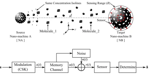
2. The Concentration-Based Molecular Communi-cations Model
As is illustrated in Fig. 1, the concentration-based MC system consists of two nano-machines, one of which, rep-resented as Nano-machine A (NA), is viewed as the source nano-machine and the other, represented as Nano-machine B (NB), is viewed as the target nano-machine. In the first stage, before the communications between NA and NB are established, the NA emits a pulse of certain molecules (denoted as Molecule 1) to enable the NB to estimate the distance. Accordingly, the NB can adjust the sampling time and set the judging condition to determine whether ‘1’ or ‘0’ is transmitted. There exist several distance esti-mation schemes, such as those shown in [18, 20, 21]. In this paper, the scheme employing the peak concentration time to estimate the distance, proposed in [18], is selected for two reasons. Firstly, this scheme is implemented based on the same propagation model as the one utilised in this pa-per, which will be introduced later. Secondly, this scheme
Noise
Sensor
a s(t) u(t) Determine
n(t)
r(t) a
Modulation (CSK)
Memory Channel
Source Nano-machineIA
[INAI]
Target Nano-machineIB
[INBI]
d
SameIConcentrationIIsolines
x z
y
Molecule_1 Molecule_2
SensingIRangeI(R)
[image:3.595.307.561.78.205.2]Sensor
Figure 1: The structure and block diagram of the MC system.
provides a sufficiently accurate estimation, and is easy to implement due to its simplicity.
In the second stage of the communication process, the NA encodes information symbols into the concentration of another kind of molecule (denoted Molecule 2). Two kinds of molecules are utilised so that the distribution of ‘estimation’ molecules will not affect that of ‘message’ molecules. To transmit bit ‘1’, the NA releases a certain amount of Molecule 2; to transmit bit ‘0’, the NA stays quiet. The NB determines incoming messages by sensing the concentration around itself to a pre-designed threshold. In contrast to existing research, the design of the thresh-old is optimised by considering previous decoded symbols, which will be introduced later. Similar to the work in [6, 7, 8, 18, 22, 23], the concentration at the NB can be considered as the concentration at the centre of the sensing sphere.
The molecule concentration in a 3D environment is ob-tained by solving Fick’s laws of diffusion, which can be re-garded as the impulse response for the 3D diffusive channel [8, 22]:
h(d, t) = 1
(4πtD)3/2exp
− d
2
4tD
, (1)
wheredis the distance between the NA and NB (inµm),
t is time (in µs), and D is the diffusion coefficient (in
µm2µs−1).
The emission process, rather than being simplified as an impulse, is modelled as a rectangular pulse given by:
s(t) =α·rect
t−T
e/2
Te
,0≤t≤Tp, (2)
where α is the emission rate (in number/µs), Te is the emission pulse duration (inµs) , Tp is the emission pulse period (in µs), and Te < Tp. If m denotes the number of molecules released per pulse, it can be deduced that
h(d, t) [16], that is:
u(d, t) =
α
4πdDerfc( d √
4tD), t≤Te
α
4πdD
erfc(√d
4tD)−erfc( d
√
4(t−Te)D
)
, t > Te (3) The NB is designed to sample the concentration at the time when theoretical concentration, u(d, t) , reaches the peak value. By deriving the equation ∂u∂t(d,t) = 0, the relationship between the distance and the sampling time
T0 can be obtained as [18]:
d2= 6D
Te
·(T0−Te)·T0·ln
T0 T0−Te
. (4)
Thus, by solving (4), the sampling time can be determined. However, molecules will not vanish within one periodTp. The remaining molecules will have an influence on the con-centration distribution of newly emitted molecules, which causes Inter-Symbol Interference (ISI). The existence time of newly emitted molecules is denoted as (I+ 1)×Tp, af-ter which the concentration referring to (3) is considered as negligible; I is called the ISI length. If this is infinite, the ISI brought in by the first pulse emission will affect all the following molecules signals; if it is finite, the channel is called a Memory Limited Channel (MLC) [24]. Thus, con-sidering the ISI, the noiseless concentration at the NB can be regarded as the sum of the current signal concentration and previous ones, that is:
uI(d, t) = I
X
i=0
u(d, t=T0+i×Tp)ak−i= I
X
i=0 uiak−i,
(5) where k represents the kth symbol from the beginning of transmission, the set {ak−i, i = 0,1, ..., I} is the binary messages sequence, the elementak−i represents the binary value of each symbol, and {ui = u(d, T0+i×Tp), i = 0,1,2, ..., I}. During the diffusion process, an additive signal-dependent noise, n(t), will also affect the concen-tration at the NB. The noise,n(t), is normally distributed with the expression given as [6, 8, 18, 19, 23]:
n(t)∼ N(0, σ2), (6)
where σ2 = 3
4πR3uI(t) =
3 4πR3
PI
i=0uiak−i. Conse-quently, referring to Fig. 1, the concentration at the NB can be derived as:
r(d, t=T0) =uI(d, t)+n(t=T0) =
I
X
i=0
uiak−i+n(t=T0).
(7) As defined in [6], the signal power and noise power of the MC system are respectively obtained by:
Wu=u20, (8)
Wn =E[n(t)2], (9)
where E[·] represents the expectation value. Given (6), the value ofE[n(t)2] can be derived as:
E[n(t)2] =E[σ2] =E
3u(t) 4πR3
= 3
4πR3E[u(t)]
= 3 4πR3E
" I X
i=0 uiak−i
#
= 3p 4πR3
I
X
i=0
ui, (10)
wherepis the probability of symbol ‘1’ transmitted. Given (8) to (10), the Signal-to-Noise-Ratio (SNR) at the NB for this MC system can be calculated as[6]:
SNR = Wu
Wn
= u
2 0 3p
4πR3
PI
i=0ui
= 4πR
3u2 0
3pPI
i=0ui
. (11)
3. Channel Analysis
The NB is designed to determine the message bits by comparing the received concentration to a pre-designed threshold η. Thus, given r(d, t = T0) representing the
sensed concentration, the judgement condition L can be expressed as:
L=r(d, t=T0)−η. (12)
The design of η has taken the influence of both previ-ous symbols and the noise into consideration, which is a method to mitigate the influence of the channel memory and noise. The method for η optimisation will be intro-duced later in this paper. When L ≥ 0, ‘1’ is decided; otherwise, ‘0’ is decided. Consideringr(d, t=T0) in (7),
the thresholdη can be designed with an expression given as [25]:
η= I
X
i=1
uiaˆk−i+τ (13)
where 0 < τ < u0, and the set {aˆk−i, i = 1,2, ..., I} is previously decoded bits within the ISI length I. If er-rors are assumed to occur independently, then previously decoded bits will not affect the decoding of the current symbol. Thus, in this case, it is assumed that ˆak−i=ak−i for i= 1,2, ..., I. By substituting (7) and (13) into (12),
Lcan be derived as:
L=n(t=T0) +aku0−τ. (14)
3.1. Bit Error Rate analysis
Error occurs only in two scenarios; when ‘0’ is transmit-ted but ‘1’ is received (named asak=0 but ˆak=1), or when ‘1’ is transmitted but ‘0’ is received (named asak=1 but ˆ
ak=0). Due to the existence of the ISI, different permu-tations of the values of{ak−i, i= 1,2, ..., I}will result in different error patterns. Each error pattern will correspond to a certain permutation of values of{ak−i, i= 1,2, ..., I}. With the ISI length equal toI, there will be 2I error pat-terns. In this work, ‘j’ denotes the error pattern index,
wherej= 1,2, ...,2I. For the error pattern ‘j’, the number of ‘1’s within the previous symbols {ak−i, i= 1,2, ..., I}is denoted as%, and the number of ‘0’s is (I−%).
(1) ak=0, but ˆak=1:
With ak = 0, to obtain the conditionL ≥0 in (14), it is required that:
n(t=T0)≥τ. (15)
Given (6), the probability for the error pattern ‘j’ with ‘0‘ transmitted can be derived by calculating the probability ofn(t=T0)≥τ, that is:
Pe0j=p%j(1−p)I−%j
Z ∞
τ 1
√
2π
1
σ0j
exp(− v 2
2σ2 0j
)dv
=p%j(1−p)I−%j
1−Φ τ
σ0j
=p%j(1−p)I−%jΦ−τ σ0j
, (16)
where σ0j =
q 3 4πR3
PI
i=1ak−iui.
(2) ak=1, but ˆak=0:
With ak = 1, to obtain the conditionL < 0 in (14), it is required that:
n(t=T0)< τ−u0. (17)
Given (6), the probability for the error pattern ‘j’ with ‘1‘ transmitted can be obtained as:
Pe1j =p%j(1−p)I−%j
Z τ−u0
−∞ 1
√
2π
1
σ1j
exp(− v 2
2σ2 1j
)dv
=p%j(1−p)I−%j
1−Φu0−τ
σ1j
=p%j(1−p)I−%jΦτ−u0 σ1j
, (18)
where σ1j =
q 3 4πR3(
PI
i=1ak−iui+u0). (3) Bit Error Rate:
The BER can be derived as:
Pe= (1−p)Pe0+pPe1
= (1−p)
2I X
j=1
Pe0j+p
2I X
j=1
Pe1j, (19)
where Pe0=
P2I
j=1Pe0j, and Pe1=
P2I
j=1Pe1j. Table 1 is an example showing the probabilities of each error pattern forI= 2.
(4) Optimise τ to minimise the error rate for each error pattern:
Aiming to achieve the minimum BER, it is required that the error rate of each pattern ‘j’ should be minimised by carefully selecting the value of τ in (16) and (18). Thus,
for a certain error pattern ‘j’,j= 1,2,3, ...,2I, the sum of error rates for either ‘1’ or ‘0’ transmitted can be expressed as:
Pej =p·Pe1j+ (1−p)Pe0j
=p%j(1−p)I−%j
p·Φτ−u0
σ1j
+ (1−p)Φ−τ
σ0j
.
(20)
Hence, the equation ∂Pej
∂τ = 0 needs to be solved:
∂Pej
∂τ =p
%j(1−p)I−%j
p·( 1
σ1j )√1
2πexp
−(u0−τ) 2
2σ2 1j
−
(1−p)( 1
σ0j )√1
2πexp
− (τ) 2
2σ2 0j
= 0. (21)
Considering 0< τ < u0, by solving (21), the optimal value
ofτ, represented asτo, can be obtained as:
τo=
−σ2
0ju0+σ0jσ1j
s
u2
0−2(σ12j−σ
2 0j)·ln
p·σ0j (1−p)σ1j
σ2
1j−σ
2 0j
.
(22)
By substituting (22) into (16), (18), and (19), the min-imised BER can be derived. Particularly, ifτ = u0
2, the
threshold is the same as the one utilised in [18, 19].
3.2. Capacity analysis
The binary input vector of the system is denoted by
X={X1, X2, ..., Xk}, and the corresponding binary out-put vector is denoted by Y ={Y1, Y2, ..., Yk}. Thus, the capacity for the memory channel can be calculated from [11]:
Capacity = lim k→∞maxp
k
X
i=1
1
kI(Xi;Yi), (23)
whereI(Xi;Yi) is the mutual information defined as [11]:
I(Xi;Yi) =H(Yi)−H(Yi|Xi)
=H[(1−p)(1−Pe0) +pPe1]
−pH(1−Pe1)−(1−p)H(1−Pe0), (24)
whereH(ξ) =−ξlog2ξ−(1−ξ) log2(1−ξ). If the channel is a memory unlimited channel with an infinite ISI length
I, the capacity can be calculated by substituting (16), (18), (19) and (24) into (23).
For an MLC with finite ISI lengthI, after theith sym-bol (i > I+ 1), the newly emitted molecular signal will be affected by the same amount (equal to I) of previous signals. Referring to (16)-(19), it can be deduced that the average error probability stays constant after theith
sym-bol (i > I+ 1). Thus, with pfixed and values ofPe0 and Pe1 being constant, it can be proven from (24) that:
Table 1: Error patterns and the probabilities for ISI lengthI= 2.
Index ISI Variance Probability of each error pattern
j ak−2 ak−1 σ0j2 σ21j
Pe0j Pe1j
(ak=0 but ˆak=1) (ak=1 but ˆak=0)
1 0 0 0 3u0
4πR3 0 (1−p)
2·
Φ(τ−u0
σ11 )
2 0 1 3u1
4πR3
3(u1+u0)
4πR3 p(1−p)·Φ(
−τ
σ02) p(1−p)·Φ(
τ−u0
σ12 )
3 1 0 3u2
4πR3
3(u2+u0)
4πR3 p(1−p)·Φ(
−τ
σ03) p(1−p)·Φ(
τ−u0
σ13 )
4 1 1 3(u1+u2)
4πR3
2
P
i=0
3ui
4πR3 p
2·
Φ(−τ
σ04) p
2·
Φ(τ−u0
σ14 )
Thus, for the MLC, the capacity calculation can be sim-plified as:
Capacity = lim k→∞maxp
k
X
i=1
1
kI(Xi;Yi)
= lim k→∞maxp
I X i=1 1
kI(Xi;Yi) +
k
X
j=I+1
1
kI(Xj;Yj)
= lim k→∞maxp
( I
X
i=1
1
kI(Xi;Yi) )
+ lim k→∞maxp
k−I
k I(XI+1;YI+1)
= 0 + max
p {I(XI+1;YI+1)} = max
p {I(XI+1;YI+1)}. (26)
By substituting (16), (18), (19) and (24) into (26), the capacity for MLC can be obtained.
3.3. Utilising the distance estimation scheme
If the distance is unknown, it is required that the dis-tance estimation process should be implemented. The NA emits a pulse of molecules, and the NB keeps sensing the concentration around itself to find the peak time of the concentration, based on which, the distance between the NA and NB can be determined. Hence, the peak time can be considered as the sampling time for the NB, denoted as
ˆ
T0. Considering (4), the distance is determined, denoted
as ˆd. Thus, during the communications stage, the sampled concentration r(t) can be derived as:
r(d, t= ˆT0) =
I
X
i=0
ak−iu(d;t= ˆT0+iTp) +n(t= ˆT0)
= I
X
i=0
ak−iudi +n(t= ˆT0), (27)
and the expression forη can be expressed as:
η= I
X
i=1
ˆ
ak−iu( ˆd, t= ˆT0+iTp) +τ0
= I
X
i=1
ˆ
ak−iu
ˆ
d
i +τ0, (28)
Similarly, it is also assumed that ˆak−i = ak−i for i = 1,2, ..., I. By substituting (27) and (28) into (12), L can be derived as:
L= I
X
i=1
ak−i(udi −u
ˆ
d
i) +akud0+n(t= ˆT0)−τ0,
=akud0+n(t=T0)−τ0+β. (29)
whereβ =PI
i=1ak−i(u
d i −u
ˆ
d
i) is substituted to make it easier to follow.
Similar to the derivation in Section 3.1, the probability for the error patternj can be obtained as:
Pedˆ1j =p%j(1−p)I−%j
1−Φu0−τ 0+β
σdˆ
1j
, (30)
Pedˆ0j =p%j(1−p)I−%j
1−Φτ 0−β
σdˆ
0j
, (31)
where
σ1dˆj =
v u u t
3 4πR3(
I
X
i=1
ak−iudi +ud0), (32)
σ0dˆj =
v u u t
3 4πR3(
I
X
i=1
ak−iudi). (33)
Correspondingly, the optimal value of τ0, represented as
τ0
o, can be derived as:
τo0 =
−(σdˆ
0j)2u0+σ ˆ
d
0jσ
ˆ
d
1j
s
u2
0−2
(σdˆ
1j)2−(σ
ˆ
d
0j)2
·ln
p·σdˆ 0j (1−p)σdˆ
1j
(σdˆ
1j)2−(σ
ˆ
d
0j)2
+β.
(34)
Thus, the BER for MC systems with the distance esti-mation scheme utilised can be computed as:
Pedˆ= (1−p)P
ˆ
d e0+pP
ˆ
d e1
= (1−p)
2I X
j=1
Pedˆ0j+p 2I X
j=1
Pedˆ1j, (35)
4. Numerical Results
In this section, numerical results for both MATLAB sim-ulations and theoretical derivations are presented. Dur-ing the simulations, the NA emits molecules periodically. Such molecules spread out and form a concentration dis-tribution in the environment. The NB samples the con-centration around itself at timeT0(or ˆT0) in each period,
based on which, the NB determines whether ‘1’s or ‘0’s are transmitted. The times of simulation trials are based on the theoretically derived results, and are designed to be sufficient to reach the required accuracy. For example, if the theoretical BER is 10−4, then 108 successive bits are
utilised to carry out the corresponding simulations. All results are presented with a common set of parameters as-signed in Table 2. These values agree with the research in [2, 6, 7, 18, 19]. Further denotation is that the optimal threshold proposed in this paper is represented as ‘OT’, and the decoding algorithm proposed in [19] is represented as ‘MSE’.
It should be noticed that when the ISI length I in-creases, not only the computation of the BER and capacity increases exponentially, but also simulations will become more complex to perform. Particularly, if I is infinite, it is impossible to obtain the required results. Thus, the channel considered herein is an MLC with a finite I. The value of I used in this paper has been greatly increased compared with all existing work, and we believe it is suffi-ciently large for the MC system analysis. If further results for larger I are required, readers could compute the BER and capacity based on (16) to (35).
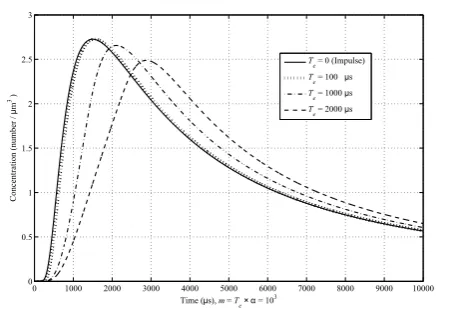
4.1. The concentration affected by the emission duration
Fig. 2 shows the change in concentration around the NB with respect to time. It can be noticed that the emis-sion duration Te is influential to the concentration distri-bution. Firstly, the rising Te will lead to the decrease in the peak concentration u0. The increase of Te means the NA emits molecules more slowly, and these molecules start to propagate to the infinite border immediately upon be-ing released. By the time the NA finishes the emission, a certain number of molecules have diffused widely in the environment. Thus, the peak concentration around the NB would be correspondingly smaller.
Secondly, the risingTewill result in the increasing con-centration tails after one pulse period, namely (ui, i = 1,2, ..., I). It has been explained that a smalleru0will be
obtained by enlarging Te. In other words, the concentra-tion gradient is gentler, and therefore after the peak time,
0 1000 2000 3000 4000 5000 6000 7000 8000 9000 10000
0 0.5 1 1.5 2 2.5 3
TimeI(µs),Im=IT
e×α=I10
3
ConcentrationI(numberI/I
µ
m
3)
T
e=I0I(Impulse)
T
e=I100Iµs
T
e=I1000Iµs
T
[image:7.595.322.557.86.242.2]e=I2000Iµs
Figure 2: The change of concentration with time for differentTeat d= 3µm.
1000 2000 5000 10000 20000 50000 100000 10−8
10−6
10−4 10−2
100
Number of molecules per pulse ( m = Te×α )
Bit Error Rate
Te = 100 µs, Theo.
Te = 1000 µs, Theo.
Te = 2000 µs, Theo.
Te = 100 µs, Simu.
Te = 1000 µs, Simu.
Te = 2000 µs, Simu.
[image:7.595.308.556.291.464.2]49000 50000 51000
Figure 3: BER Vs. mfor differentTewithI= 20 andd= 3µm.
molecules will diffuse to the infinite border in a lower rate, which means the attenuation of the concentration will be correspondingly slower. As a consequence, the concentra-tion tails will be enlarged.
Referring to (11), either the decrease of the peak con-centration (u0) or the increase of the tail (ui, i= 1,2, ..., I) will lead to a smaller SNR. Then, it can be deduced that the MC system with a largeTe will exhibit a worse per-formance, which agrees with the curves shown in Figs. 3 to 5.
4.2. Channel performance analysis for OT decoding algo-rithm
Table 2: Simulation parameters
1. The radium of the NB R 0.5µm 2. The distance between NA and NB d 2∼4µm 3. The diffusion coefficient D 10−3µm2µs−1 4. The emission duration Te 100∼2000µs 5. The pulse period Tp 5000µs 6. The number of transmitted molecules m 103∼105
1000 2000 5000 10000 20000 50000 100000
10−10 10−8 10−6 10−4 10−2 100
Numberhofhmoleculeshperhpulseh(hm = T e×α)
BithErrorhRate
I=h 2h,hTheo.
I=h10,hTheo.
I=h15,hTheo.
I=h20,hTheo.
I=h25,hTheo.
I=h 2h,hSimu.
I=h10,hSimu.
I=h15,hSimu.
I=h20,hSimu.
I=h25,hSimu.
[image:8.595.55.286.181.350.2]49000 50000 51000
Figure 4: BER Vs. mfor differentIwithTe= 1000µs andd= 3µm.
10000 2000 5000 10000 20000 50000 100000
5 10 15 20 25
Number of molecules per pulse ( )
Signal
−
to
−
Noise
−
Ratio ( SNR ) in dB
0.2 0.4 0.6 0.8 1
Capacity
T
e= 1000 µs,
I= 10, SNR
T
e= 1000 µs,
I= 20, SNR
T
e= 2000 µs,
I= 10, SNR
T
e= 1000 µs,
I= 10, Capacity
T
e= 1000 µs, I= 20, Capacity
T
e= 2000 µs, I= 10, Capacity
m = Te × α
Figure 5: SNR and capacity Vs. m for different I and Te with d= 3µm.
To be specific, in Figs. 3 to 5, increasing m will help the system to suffer less from errors and achieve a higher capacity. The reason is that with more molecules emit-ted per pulse, the system will have a stronger resistance against the noise and ISI. Referring to (3)-(11), amplify-ing m leads to a larger SNR, which guarantees a better performance.
The change inTewill also affect the BER and capacity of the system. In Figs. 3 and 5, decreasing Te leads to a smaller BER and higher capacity. As is explained in Section 4.1, the reduction ofTebrings about a larger SNR. Thus, if the NA emits molecules as fast as possible, the channel performance can be enhanced.
Another factor that influences the system is the ISI length. Even though the influence of the ISI has been mit-igated by using the decoding method described by (12) to (14), it can be deduced from (6) that the remaining concen-trations of previous bits will contribute to the noise effect. Consequently, the ISI will still affect the channel perfor-mance. If the ISI can be further alleviated, a smaller BER and higher capacity will be obtained. This shows agree-ment with the results in Figs. 4 and 5 that decreasing
I also results in a larger SNR because molecules vanish more quickly so that less influence will be brought onto the upcoming signals. Moreover, as is also clearly shown here, there is no significant difference in performance be-tween I = 15,20,and 25. Thus, considering the fact that with I rising, the complexity of both the computation of BER and capacity and MATLAB simulations increases ex-ponentially,I = 20 is sufficiently large for system perfor-mance analysis.
It should also be noticed that the simulated BER is slightly higher than the theoretical BER even if the de-viation is almost negligible. The main reason of the differ-ence herein is that the assumption that errors occur inde-pendently for theoretical derivation does not hold during simulations. In other words, when decoding the bitak, for theoretical derivation, it is assumed that ˆak−i =ak−i for
i= 1,2, ..., I; while for simulations, one wrongly decoded bit will affect the decoding of next several symbols. Errors therefore occur in succession, which is calledError
Propa-gation. Additionally, during simulations, there is a chance
that the concentration may rise to a high value and takes time to recover to a normal level, which also affects the de-coding of next several symbols. This also causes the Error Propagation, leading to a higher BER for simulations.
An important but not intuitive feature shown through-out Figs. 3 to 5 is that no matter how parameters are selected, the performance almost remains the same if the system SNR remains constant. An example is shown in Fig. 6 where the BER for MC systems with different pa-rameters is presented. As is illustrated there, although the assignment of parameters varies, the difference in the error probabilities of MC systems with the same SNR is so small that it can be neglected. Therefore, the SNR, defined in (11), can be considered as a reasonable metric to evaluate the diffusive concentration-based MC system performance.
[image:8.595.47.288.399.553.2]10 12 14 16 18 20 10−8
10−6
10−4
10−2
100
Signal − to − Noise − Ratio (SNR) in dB
Bit Error Rate (BER)
d = 2 µm, T
e= 1000 µs, I= 20
d = 3 µm, T
e= 1000 µs, I= 20
d = 3 µm, T
e= 1000 µs, I= 10
d = 3 µm, T
e= 2000 µs, I= 20
15 16 17
0 1 2 3 4 5x 10
[image:9.595.325.554.85.241.2]−3
Figure 6: BER Vs. SNR for different parameter assignment.
0 5 10 15 20 25
10−8
10−6
10−4
10−2
100
SignalO−OtoO−ONoiseO−ORatioO(OSNRO)OinOdBO
BitOErrorORateO(OBERO)
0.4 0.6 0.8 1
Capacity
[image:9.595.56.287.86.241.2]OTO,OBER MSE,OBER OTO,OCapacity MSE,OCapacity
Figure 7: Performance comparisons between OT and MSE withI= 20,Te= 1000µs, andd= 3µm.
4.3. Channel performance comparisons between OT and MSE decoding algorithms
In Fig. 7, the performance enhancement by using OT rather than MSE is presented. For MSE, the parameterτ
of the threshold η is set to be τ = u0
2, while for OT, the
value ofτis optimised according to different error patterns. By coordinating τ, the BER for each error pattern has been minimised. Consequently, the concentration-based MC system tends to enjoy a lower error rate and a better maximum reliable transmission rate. However, this perfor-mance improvement is brought in at the cost of a higher requirement on the complexity of the NB. As expressed in (22), the optimal value ofτ keeps changing through the communications process, and requires the NB to determine the corresponding optimal τo within the time less than a pulse periodTp, which may exceed the capability of nano-machines. Hence, when choosing the decoding algorithms, not only should the system performance be taken into ac-count, but also the complexity of nano-machines needs to be considered.
2 2.5 3 3.5 4
10−7
10−6
10−5
10−4
10−3
10−2
10−1
The distance between the TA and TB, d( μm )
Bit Error Rate ( BER )
−0.4
−0.2 0 0.2 0.4 0.6
Av
er
age
d
is
tan
ce
d
ev
iat
ion
d
d
(
)
BER for averaged
BER ford=d
BER deviation between averagedandd
Averaged-d
-μ
m
˄ ˄
˄
˄
[image:9.595.56.288.289.443.2]˄
Figure 8: BER and the estimation deviation ( ˆd-d) Vs. dwithTe=
1000µs andI= 20. The dashed line between two ‘∗’ or ‘×’ symbols represents the variation range of the BER or deviation.
2 2.5 3 3.5 4
0.6 0.7 0.8 0.9 1
The distance between the Tx and Rx,d(µm)
C
a
p
a
ci
ty
5 10 15 20 25
Capacity for average ˆd
Capacity for ˆd=d
SNR
Figure 9: SNR and capacity Vs. dwithTe = 1000µs andI = 20.
The dashed line between two ‘×’ symbols represents the variation range of the Capacity.
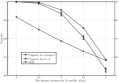
4.4. Channel performance analysis with the distance un-known
The performance evaluation with the distance estima-tion scheme implemented is presented in Figs. 8 and 9. As is clearly shown, with the distancedgetting larger, the system tends to suffer from a higher BER and correspond-ingly lower capacity. Whendincreases, it can be deduced from (3) that fewer molecules will arrive at the NB. In this case, any slight change of the concentration will sig-nificantly affect the decoding process of the NB, which can be also explained as the system has a smaller SNR accord-ing to (3) through (11). Thus, the system will have a weak resistance against the influence of the noise and ISI.
[image:9.595.308.558.302.477.2]estimation accuracy, there will be less error occurrence in the system. An obvious method to enhance the system performance is to increase the SNR of the system. With a larger SNR, not only can the estimation be more accurate, but also the system will suffer less from the impact of the channel noise and memory. It can be deduced from Section 4.2 that three options can be applied to increase the SNR, i.e., increasing m, decreasing Te, and further mitigating the influence of the ISI.
5. Conclusions
In this paper, a new decoding algorithm with an opti-mised threshold is proposed for a concentration-based MC system, which has been refined by taking the TN emission process into consideration. Based on this model, an infor-mation theoretical approach has been proposed to evaluate the system performance in terms of the BER and channel capacity. Simulations have also been carried out to ver-ify the accuracy of these analytical formulations, and the cause of the deviation between the theoretically derived and simulated results has been explained. Numerical re-sults illuminate that the BER and capacity are highly de-pendent on the number of molecules emitted per pulse (m), the emission duration (Te), the ISI length (I) and the distance between the NA and NB (d). System per-formance for OT and MSE decoding techniques is com-pared to show the superiority of this new decoding al-gorithm. Moreover, this is the first investigation on the performance of MC systems with the distance unknown for nano-machines. Comparisons between distance-pre-known systems and distance-undistance-pre-known systems have been made, and results reveal that the performance can be en-hanced by three methods, releasing more molecules, re-leasing molecules faster, and mitigating the influence of the ISI and the noise.
References
[1] Atakan B, Akan OB. An information theoretical approach for molecular communication. In: International Conference on Bio-Inspired Models Networks, Information, and Computing Sys-tems. 2007, p. 33–40. doi:10.1109/BIMNICS.2007.4610077. [2] Pierobon M, Akyildiz IF. Capacity of a diffusion-based
molecular communication system with channel memory and molecular noise. IEEE Transactions on Information Theory 2013;59(2):942–954. doi:10.1109/TIT.2012.2219496.
[3] Eckford AW. Achievable information rates for molecu-lar communication with distinct molecules. In: Interna-tional Conference on Bio-Inspired Models Networks, Infor-mation, and Computing Systems. 2007, p. 313–315. doi: 10.1109/BIMNICS.2007.4610135.
[4] Mosayebi R, Arjmandi H, Gohari A, Nasiri-Kenari M, Mitra U. Receivers for diffusion-based molecular communication: Ex-ploiting memory and sampling rate. IEEE Journal on Se-lected Areas in Communications 2014;32(12):2368–2380. doi: 10.1109/JSAC.2014.2367732.
[5] Kim NR, Chae CB. Novel modulation techniques using isomers as messenger molecules for nano communication networks via diffusion. IEEE Journal on Selected Areas in Communications 2013;31(12):847–856. doi:10.1109/JSAC.2013.SUP2.12130017.
[6] Kilinc D, Akan OB. Receiver design for molecular communi-cation. IEEE Journal on Selected Areas in Communications 2013;31(12):705–714. doi:10.1109/JSAC.2013.SUP2.1213003. [7] ShahMohammadian H, Messier GG, Magierowski S.
Op-timum receiver for molecule shift keying modulation in diffusion-based molecular communication channels. Nano Communication Networks 2012;3(3):183 –195. doi: http://dx.doi.org/10.1016/j.nancom.2012.09.006.
[8] Llatser I, Cabellos-Aparicio A, Pierobon M, Alarcon E. De-tection techniques for diffusion-based molecular communica-tion. IEEE Journal on Selected Areas in Communications 2013;31(12):726–734. doi:10.1109/JSAC.2013.SUP2.1213005. [9] Atakan B, Akan OB. On channel capacity and error
compen-sation in molecular communication. In: Transactions. on Com-putational Systems Biology X; vol. 5410 of Lecture Notes in Computer Science. Springer Berlin Heidelberg; 2008, p. 59–80. doi:10.1007/978-3-540-92273-5-4.
[10] Kuran MS, Yilmaz HB, Tugcu T, Akyildiz IF. Modulation techniques for communication via diffusion in nanonetworks. In: IEEE International Conference on Communications (ICC). 2011, p. 1–5. doi:10.1109/icc.2011.5962989.
[11] Nakano T, Okaie Y, Liu JQ. Channel model and capac-ity analysis of molecular communication with brownian mo-tion. IEEE Communications Letters 2012;16(6):797–800. doi: 10.1109/LCOMM.2012.042312.120359.
[12] Moore MJ, Suda T, Oiwa K. Molecular communica-tion: Modeling noise effects on information rate. IEEE Transactions on NanoBioscience 2009;8(2):169–180. doi: 10.1109/TNB.2009.2025039.
[13] Singhal A, Mallik RK, Lall B. Molecular communication with brownian motion and a positive drift: performance analy-sis of amplitude modulation schemes. IET Communications 2014;8(14):2413–2422. doi:10.1049/iet-com.2013.0939.
[14] Chahibi Y, Akyildiz IF. Molecular communication noise and capacity analysis for particulate drug delivery systems. IEEE Transactions on Communications 2014;62(11):3891–3903. doi: 10.1109/TCOMM.2014.2360678.
[15] Singhal A, Mallik RK, Lall B. Effect of molecular noise in diffusion-based molecular communication. IEEE Wireless Communications Letters 2014;3(5):489–492. doi: 10.1109/LWC.2014.2345756.
[16] Mahfuz MU, Makrakis D, Mouftah HT. On the characterization of binary concentration-encoded molecular communication in nanonetworks. Nano Communication Networks 2010;1(4):289 – 300. doi:http://dx.doi.org/10.1016/j.nancom.2011.01.001. [17] Yilmaz HB, Chae CB. Simulation study of molecular
communication systems with an absorbing receiver: Mod-ulation and ISI mitigation techniques. Simulation Mod-elling Practice and Theory 2014;49:136 – 150. doi: http://dx.doi.org/10.1016/j.simpat.2014.09.002.
[18] Wang X, Higgins MD, Leeson MS. Distance estimation schemes for diffusion based molecular communication sys-tems. IEEE Communications Letters 2015;19(3):399–402. doi: 10.1109/LCOMM.2014.2387826.
[19] Wang X, Higgins MD, Leeson MS. Relay analysis in molecular communications with time-dependent concentration. IEEE Communications Letters 2015;19(11):1977–1980. doi: 10.1109/LCOMM.2015.2478780.
[20] Moore MJ, Nakano T, Enomoto A, Suda T. Measuring distance from single spike feedback signals in molecular communication. IEEE Transactions on Signal Processing 2012;60(7):3576–3587. doi:10.1109/TSP.2012.2193571.
[21] Huang JT, Lai HY, Lee YC, Lee CH, Yeh PC. Distance estimation in concentration-based molecular communications. In: IEEE Global Communications Conference (GLOBECOM). 2013, p. 2587–2591. doi:10.1109/GLOCOM.2013.6831464. [22] Ahmadzadeh A, Noel A, Schober R. Analysis and
de-sign of multi-hop diffusion-based molecular communication networks. IEEE Transactions on Molecular , Biological and Multi-Scale Communications 2015;(1)(6):144–157. doi: 10.1109/TMBMC.2015.2501741.
[23] Pierobon M, Akyildiz IF. Diffusion-based noise analysis for molecular communication in nanonetworks. IEEE Trans-actions on Signal Processing 2011;59(6):2532–2547. doi: 10.1109/TSP.2011.2114656.
[24] Aminian G, Arjmandi H, Gohari A, Kenari MN, Mitra U. Ca-pacity of LTI-Poisson channel for diffusion based molecular com-munication. In: IEEE International Conference on Communica-tions (ICC). 2015 p. 1060–1065. doi:10.1109/ICC.2015.7248463. [25] Rodriguez-Henriquez F, Rocha-Perez JM, Silva-Martineze J. Performance of a decision feedback demodulator in a time-dispersive channel for ISI cancellation and its implementation in switched-capacitor technique. In: IEEE International Sym-posium on Personal, Indoor and Mobile Radio Communications (PIMRC). 1999, p. 1–5.
Xiayang Wang received the
de-gree of Bachelor of Science majoring in Opto-information Science and Technology from the Department of Optoelectronics Science and Technology in Huazhong University of Science and Technology, China, in 2011. In 2013, he graduated from the Department of Electronics at the University of York, receiving a First Class Honors MSc degree in Communications Engineering. Xiayang then moved to the University of Warwick where he is currently working towards his PhD in Nano-communications.
Yi Lu received the degree of
Bachelor of Engineering with First Class Honors in Electronic Engi-neering from University of Central Lancashire, UK, in 2011. And then she obtained a Master degree of Engineering with Distinction in Electronic Engineering from University of Sheffield, UK, in 2012. She is currently a scholarship student pursuing a PhD study in Nano-communications at University of Warwick.
Matthew D. HigginsMatthew
Higgins received his MEng in Electronic and Communications Engineering and his PhD in Engineering from the School of Engineering at the University of Warwick in 2005 and 2009 respec-tively. Remaining at the University of Warwick, he then progressed through several Research Fellow positions, in association with some of the UKs leading defence and telecommunications com-panies before undertaking two years as a Senior Teaching Fellow in Telecommunications, Electrical Engineering and Computer Science subjects. In July 2012, Dr Higgins was promoted to the position of Assistant Professor where
his research focused on Optical, Nano, and Molecular Communications. Whilst is this position, Dr Higgins set up the Vehicular Communications Research Laboratory which aimed to enhance the use of communications systems within the vehicular Space. As of March 2016, Dr Higgins was appointed as an Associate Professor at WMG working in the area of Connected and Autonomous Vehicles. Dr Higgins is a Senior Member of the IEEE, SMIEE, a member of the IEEE Communications Soci-ety, COMSOC, and a Fellow of the Higher Education Academy, FHEA.
Mark S. Leesonreceived the