Wave sensitivity analysis for periodic and arbitrarily complex composite structures

Wave sensitivity analysis for periodic and arbitrarily

complex composite structures

D. Chronopoulosa_{, M. Collet}b_{, M. Ichchou}c

a

Institute for Aerospace Technology &The Composites Group, The University of Nottingham, NG7 2RD, UK

b

LTDS, UMR-CNRS 5513, 36 Avenue Guy de Collongue, 69130 Ecully, France

c

Ecole Centrale de Lyon, 36 Avenue Guy de Collongue, 69130 Ecully, France

Abstract

Purpose: This paper presents the development of a numerical continuum-discrete approach for computing the sensitivity of the waves propagating in

periodic composite structures. The work can be directly employed for

eval-uating the sensitivity of the structural dynamic performance with respect to

geometric and layering structural modifications.

Design/methodology/approach: A structure of arbitrary layering and geometric complexity is modelled using solid FE. A generic expression for

computing the variation of the mass and the stiffness matrices of the structure

with respect to the material and geometric characteristics is hereby given.

The sensitivity of the structural wave properties can thus be numerically

de-termined by computing the variability of the corresponding eigenvalues for

the resulting eigenproblem. The exhibited approach is validated against the

FD method as well as analytical results.

Findings: An intense wavenumber dependence is observed for the sensitivity

results of the sandwich structure. This exhibits the importance and potential

of the presented tool with regard to the optimization of layered structures for

specific applications. The model can also be used for computing the effect of

the inclusion of smart layers such as auxetics and piezoelectrics.

Originality/value: The paper presents the first continuum-discrete ap-proach specifically developed for accurately and efficiently computing the

sensitivity of the wave propagation data for periodic composite structures

ir-respective of their size. The considered structure can be of arbitrary layering

and material characteristics as FE modelling is employed.

Keywords: Sensitivity analysis, Wave propagation, Composite structures

1. Introduction

Layered and complex structures are nowadays widely used within the

aerospace, automotive, construction and energy sectors with a general

in-crease tendency. The wave propagation data for such structures are often

employed for energy harvesting, vibration control, health monitoring and

vibroacoustic transmission modelling purposes. Optimizing the layer

char-acteristics of such structures for certain objectives is often a challenging task

due to the large number of varying parameters to be considered as well as

due to the lack of exact modelling approaches. The same it true about taking

into account for the effect of these parametric uncertainties on the structural

behaviour.

The numerical analysis of wave propagation within periodic structures

was firstly considered in the pioneering work of the author of [1]. The work

a structured linearization method using state space eigenvalue problem for

large matrices among other considerations for smoothening the solution of

wave propagation in periodic structures. The WFE method was introduced

in [4, 5] in order to facilitate the post-processing of the eigenproblem

solu-tions and further improve the computational efficiency of the method. The

vibration of a uniform waveguide using the same technique was investigated

by the authors of [6, 7, 8]. The WFE method for two dimensional structures

was introduced in [9] . The same method was used in [10] in order to

com-pute the dynamic response of two dimensional infinite structures. The WFE

has recently found applications in predicting the vibroacoustic and dynamic

performance of composite panels and shells [11, 12, 13, 14, 15, 16, 17] , with

pressurized shells [18, 19] and complex periodic structures [20, 21, 22] having

been investigated. The variability of acoustic transmission through layered

structures [23, 24], as well as wave steering effects in anisotropic composites

[25] have been modelled through the same methodology.

Structural sensitivity analysis is of great importance for understanding

the overall impact of a design parameter variation to the structural

perfor-mance which is to be optimised. Accurate sensitivity models are an important

tool for design optimization, system identification as well as for statistical

me-chanics analysis. Many authors [26, 27, 28, 29] have been focusing on the

eigenvalue derivative analysis of a structural system. With regard to the

variability analysis of the waves travelling within a structural medium the

conducted work has been mainly focused on deriving expressions [30, 31] of

the stochastic wave parameters from analytical models. In [32] the authors

numerical approaches the authors in [33] used Bloch’s theorem in

conjunc-tion with the FE method in order to calculate the sensitivity of the acoustic

waves within an auxetic honeycomb, while with regard to the computation

of the variability of the propagating waves the authors in [34, 35] have

pre-sented a stochastic WFE method approach for computing the stochastic wave

propagation in one dimensional media.

In this paper a continuum-discrete approach for efficiently computing the

sensitivity of the wave propagation data for periodic structures is presented.

The considered structure can be of arbitrary layering and material

character-istics as FE modelling is employed. The effect of local parameter variation

(e.g. varying the stiffener thickness or adding mass to a single location) can

also be considered. The sensitivities of the mass and stiffness matrices for a

solid FE are computed with respect to any structural parameter including

the material characteristics and the thickness of the element. The sensitivity

of the propagating structural waves can thus be numerically determined. The

exhibited approach is validated against the FD method as well as analytical

results.

The paper is organized as follows: In Sec.2 the formulation of the

sensi-tivity of the waves propagating within the periodic structure is elaborated.

More precisely in Sec.2.1 a general approach for two dimensional waveguides

is adopted while in Sec.2.2 a more efficient approach for one dimensional

waveguides is considered. In Sec.3 the method is validated by comparison to

analytical results for a metallic waveguide as well as by comparison to a FD

approach for a layered sandwich waveguide. Conclusions on the presented

the stiffness and mass matrices of a solid FE are presented in the Appendix A.

2. Sensitivity of the wave propagation data

2.1. General formulation

2.1.1. Formulation of the PST for an arbitrary structural segment

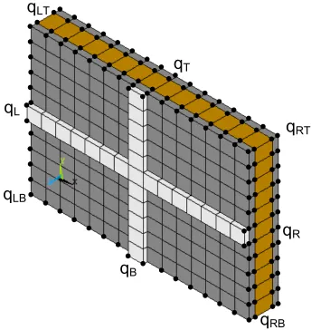
A periodic segment of a panel having arbitrary layering and complexity

is hereby considered (see Fig.1) with lx, ly its dimensions in the x and y

directions respectively. The segment is modelled using a conventional FE

software. The mass and stiffness matrices of the segment M and K are

extracted and the DoF set qis reordered according to a predefined sequence such as:

q={qI qB qT qL qR qLB qRB qLT qRT}⊤ (1)

corresponding to the internal, the interface edge and the interface corner DoF

(see Fig.1). The free harmonic vibration equation of motion for the modelled

segment is written as:

[K−ω2

M]q=0 (2)

The analysis then follows as in [36] with the following relations being

as-sumed for the displacement DoF under the passage of a time-harmonic wave:

qR =e−iεxqL, qT =e−iεyqB

qRB =e−iεxqLB, qLT=e−iεyqLB, qRT =e−iεx−iεyqLB

(3)

with εx andεy the propagation constants in the xandydirections related to

the phase difference between the sets of DoF. The wavenumbers kx, ky are

directly related to the propagation constants through the relation:

q

q

q

q

q

q

q

q

Considering Eq.(3) in tensorial form gives: q=                       

I 0 0 0

0 I 0 0

0 Ie−iεy _{0 0}

0 0 I 0

0 0 Ie−iεx ₀

0 0 0 I

0 0 0 Ie−iεx

0 0 0 Ie−iεy

0 0 0 Ie−iεx−iεy

                      

x=Rx (5)

with x the reduced set of DoF: x = {qI qB qL qLB}⊤. The equation of

free harmonic vibration of the modelled segment can now be written as:

[R∗_KR−ω2_R∗_{MR]x=0 (6)}

with ∗ _{denoting the Hermitian transpose. The most practical procedure for}

extracting the wave propagation characteristics of the segment from Eq.(6)

is injecting a set of assumed propagation constants εx, εy. The set of these

constants can be chosen in relation to the direction of propagation towards

which the wavenumbers are to be sought and according to the desired

reso-lution of the wavenumber curves. Eq.(6) is then transformed into a standard

eigenvalue problem and can be solved for the eigenvector x which describe the deformation of the segment under the passage of each wave type at an

angular frequency equal to the square root of the corresponding eigenvalue

A complete description of each passing wave including its x and y

direc-tional wavenumbers and its wave shape for a certain frequency is therefore

acquired. It is noted that the periodicity condition is defined modulo 2π,

therefore solving Eq.(6) with a set of εx,εy varying from 0 to 2π will suffice

for capturing the entirety of the structural waves. Further considerations

on reducing the computational expense of the problem are discussed in [36].

It should be noted that only propagating waves will be considered in the

subsequent analysis. Evanescent waves can also be captured by introducing

imaginary values for εx, εy however the precise computation of these waves

would require a very fine resolution of the propagation constants, drastically

increasing the computational effort.

2.1.2. Parametric sensitivity

It is noted that matrices K = R∗_{KR and M = R}∗_{MR in Eq.(6) are}

Hermitian therefore their resulting eigenvalues are real and the eigenvectors

will be orthogonal. Assuming the known eigenvalueλ0iand the corresponding

eigenvectorx0i for the problem described in Eq.(6), then the following is true

K0x0i =λ0iM0x0i (7)

Now if matricesK0,M0 are changed by a small amount, sayδK,δM then the eigenvalue λ0i and the corresponding eigenvector x0i will also be perturbed

so that

K=K0+δK

M=M0 +δM λi =λ0i+δλi xi =x0i+δxi

A direct consequence of the orthogonality of the eigenvectors is that

x⊤₀kM0x0i =δki (9)

with δk

i the Kronecker delta function. Substituting Eq.(8) into Eq.(7), we

get

(K0+δK)(x0i+δxi) = (λ0i+δλi)(M0 +δM)(x0i +δxi) (10)

then expanding and using Eq.(7) we can write

δKx0i+K0δxi+δKδxi =

λ0iM0δxi+λ0iδMx0i+δλiM0x0i +λ0iδMδxi +δλiδMx0i +δλiM0δxi+δλiδMδxi

(11)

and removing the higher-order terms simplifies to

K0δxi+δKx0i =λ0iM0δxi+λ0iδMx0i+δλiM0x0i (12)

The orthogonality properties of the unperturbed eigenvectors in Eq.(6) allow

for using them as a basis for expressing the perturbed eigenvectors. That is

the perturbation of the eigenvector x0i can be expressed as

δxi =

N X

k=1

ǫikx0k (13)

with ǫik small unknown constants. Substituting Eq.(13) into Eq.(12) gives

K0

N X

k=1

ǫikx0k+δKx0i =λ0iM0

N X

k=1

ǫikx0k+λ0iδMx0i+δλiM0x0i (14)

which can also be written as

N X

k=1

ǫikK0x0k+δKx0i =λ0iM0

N X

k=1

Making use of Eq.(7) it is true that

N X

k=1

ǫikλ0kM0x0k+δKx0i =λ0iM0

N X

k=1

ǫikx0k+λ0iδMx0i+δλiM0x0i (16)

Again due to the orthogonality of the eigenvectors in Eq.(9), the summations

can be removed by left multiplying by x⊤

0i, therefore

x⊤

0iǫiiλ0iM0x0i+x⊤0iδKx0i =λ0ix⊤0iM0ǫiix0i+λ0ix⊤0iδMx0i +δλix⊤0iM0x0i

(17)

and eliminating the equal terms gives

x⊤

0iδKx0i =λ0ix⊤0iδMx0i+δλix⊤0iM0x0i (18)

Rearranging the expression with regard to δλi we get

δλi = x⊤

0i(δK−λ0iδM)x0i x⊤

0iM0x0i

(19)

However, because of Eq.(9) the expression of the eigenvalue perturbation is

given as

δλi =x⊤0i(δK−λ0iδM)x0i (20)

When the partial derivatives of K,M with regard to a design parameter β are known then the sensitivity of an eigenvalue λi to this design parameter

will be equal to

∂λi

∂β =x

⊤

0i

∂K

∂β −λ0i ∂M

∂β

x0i (21)

The global mass and stiffness matrices M,K of the structural segment

are formed by adding the local mass and stiffness matrices of individual

FEs. Therefore it can be concluded that when the expression of the partial

derivatives for every local mass and stiffness matrix ∂m ∂β ,

∂k

the expressions for the global matrices ∂M ∂β ,

∂K

∂β can be derived simply by adding the expressions of the local matrices together. Eq.(21) can therefore

be written as:

∂λi

∂β =x

⊤

0i

R∗∂K

∂βR−λ0iR

∗∂M

∂β R

x0i (22)

It is known however that ∂λi ∂β =

∂(ω2

i)

∂β , therefore

∂λi

∂β = ∂(ω2

i)

∂β =

∂(ω2

i)

∂ωi

∂β ∂ωi

= 2ωi

∂ωi

∂β (23)

Eq.(22) can therefore be written as:

∂ωi

∂β =

x⊤

0i

R∗∂K

∂βR−λ0iR∗ ∂M

∂βR

x0i

2ωi

(24)

with ωi the angular frequency at which the set ofεx,εy is true for the iwave

type described by the x0i deformation. The generic symbolic expressions

of the m,k matrices for an orthotropic structural segment modelled with a linear solid FE is given in Appendix A. The wavenumber sensitivity ∂ki

∂β can be deduced as

∂ki

∂β =− ∂ki

∂ωi

∂ωi

∂β =− 1 cg,i

∂ωi

∂β (25)

with cg,i =

∂ωi

∂ki

the group velocity associated with the wave type i at

fre-quency ωi which can be evaluated by avoiding any numerical differentiation

as exhibited in [37].

2.2. Transfer matrix formulation

2.2.1. Condensation process

When wave propagation is considered only in thexdirection, the problem

structural segment is again partitioned, this time with regard to its left/right

sides and internal DoF



   

DLL DLI DLR DIL DII DIR DRL DRI DRR

              qL qI qR          =          fL 0 fR          (26)

with q the displacement and f the force vectors. Using a Guyan type con-densation for the internal DoF the problem can be expressed as





DLL−DLID−_II1DIL DLR−DLID−_II1DIR DRL−DRID−1

IIDIL DRR−DRID−

1 IIDIR      qL qR    =    fL fR    (27)

Assuming that no external forces are applied on the segment the displacement

continuity and force equilibrium equations at the interface of two consecutive

periodic segments s and s+ 1 give

qs+1

L =qsR fs+1

L =−f s R

(28)

Using Eqs.(27),(28) the relation of the displacements and forces of the left

and right sides of the segment can be written as

 

 qs_L+1 fs+1

L    =T    qs L fs L    (29)

and the expression of the symplectic transfer matrix T can be written as

T= 



D11 D12

D21 D22



with

D11=−(DLR−DLID−_II1DIR)−1(DLL−DLID−_II1DIL)

D12= (DLR−DLID−_II1DIR)−1

D21=−DRL+DRID−II1DIL+ (DRR−DRID−II1DIR)(DLR−DLID−II1DIR)−1(DLL−DLID−II1DIL)

D22=−(DRR−DRID−_II1DIR)(DLR−DLID−_II1DIR)−1

(31)

Free wave propagation is described by the eigenproblem

γ  

 qs

L fs

L  

 =T

 

 qs

L fs

L  



(32)

whose solution γi is related to the structural wavenumber kxi by

kxi=−

ln(γi)

ilx

(33)

2.2.2. Parametric sensitivity

Assuming the known eigenvalue γ0i and the corresponding eigenvector

z0i =  

 q0i

f0i  



for the problem described in Eq.(32), then the following is

true

γ0iz0i =T0z0i (34)

Now if the matrix T0 is changed by a small amount, say δT then the eigen-value γ0i and the corresponding eigenvector z0i will also be perturbed so

that

(γ0i+δγi)(z0i+δzi) = (T0+δT)(z0i+δzi) (35)

Expanding we have

However using Eq.(34) and removing the higher-order terms eventually

sim-plifies the relation to

γ0iδzi+δγiz0i =T0δzi+δTz0i (37)

The symplectic orthogonality properties [5] of the unperturbed eigenvectors

of T0 suggest that if γi is an eigenvalue of T0 with the corresponding right eigenvector zi, then 1/γi will also be an eigenvalue of T0 with a corre-sponding left eigenvector yi = ziJn, with Jn a 2n × 2n matrix given as

Jn = 



0 In

−In 0



 . The following will also apply if the eigenvectors are

appropriately scaled

Y⊤0Z0 =I (38)

and

Y⊤

0T0Z0 =Γ0 (39)

with Γ0 the diagonal matrix containing the eigenvalues of T₀, while

Y0 = [y01y02· · ·y0n] (40)

is the matrix containing the left eigenvectors of T0 and

Z0 = [z01z02· · ·z0n] (41)

the matrix containing the right eigenvectors of T0. The orthogonality prop-erty allows for expressing the perturbation of the eigenvector z0i as

δzi =

N X

k=1

with ǫik small unknown constants. Substituting Eq.(42) into Eq.(37) and

making use of Eq.(34) once again gives

γ0i N X

k=1

ǫikz0k+δγiz0i = N X

k=1

ǫikγ0kz0k+δTz0i (43)

and due to Eq.(38), the summations can be removed by left multiplying by

y⊤

0i, therefore

y⊤

0iǫiiγ0iz0i+y0⊤iδγiz0i =y0⊤iǫiiγ0iz0i+y0⊤iδTz0i (44)

Eliminating the equal terms gives

y⊤

0iδγiz0i =y0⊤iδTz0i (45)

Due to the orthogonality of the eigenvectors it is true that

y⊤0iz0i = 1 (46)

therefore the expression of the eigenvalue perturbation δγi as a function of

the transfer matrix perturbation δT can be written as

δγi =y⊤0iδTz0i (47)

When the partial derivative of T with regard to a design parameter β is known then the sensitivity of an eigenvalue γi to β is equal to

∂γi

∂β =y

⊤ i

∂T

∂βzi (48)

It is known however that ∂γi ∂β =

∂(e−ikxilx)

∂β , therefore

∂(e−ikxilx₎

∂kxi

∂β ∂kxi

=−ilxe−ikxilx

∂kxi

Eq.(48) can therefore be written as:

∂kxi

∂β =

1

−ilxe−ikxilx y⊤i

∂T

∂βzi (50)

The symbolic expression of the ∂k ∂β,

∂m

∂β matrices for a structural segment modelled with a linear solid FE can be derived using the expressions given

in Appendix A.. The corresponding expression of the DSM in Eq.(27) can

therefore be directly computed. The symbolic expression of T as well as of the sensitivity ∂T

∂β can thereafter be derived using Eq.(31). It should be noted that due to the inversion and multiplication of DSM partitions involved

in Eq.(31), this approach tends to be less computationally efficient than the

one presented in Sec.2.1.2, especially for large structural segments.

3. Numerical case studies

Two case studies are presented below in order to validate the presented

work. In the first case a metallic monolayer panel is modelled by the

pre-sented approach and the results on the sensitivity of the propagating waves

are compared to the values derived by the CPT. In the second case study a

sandwich panel comprising facesheets of different thicknesses is modelled and

the results are validated through the FD method. Both cases were modelled

using the approach presented in Sec.2.1. All computations were conducted

using the R2013a version of MATLABr_.

3.1. Monolayer panel

A metallic single layer panel is hereby modelled. The panel has a

Young’s modulus E = 70GPa and a Poisson’s ratio equal to v=0.1. Three

equidimensional FE are used in order to model the structure in the sense of

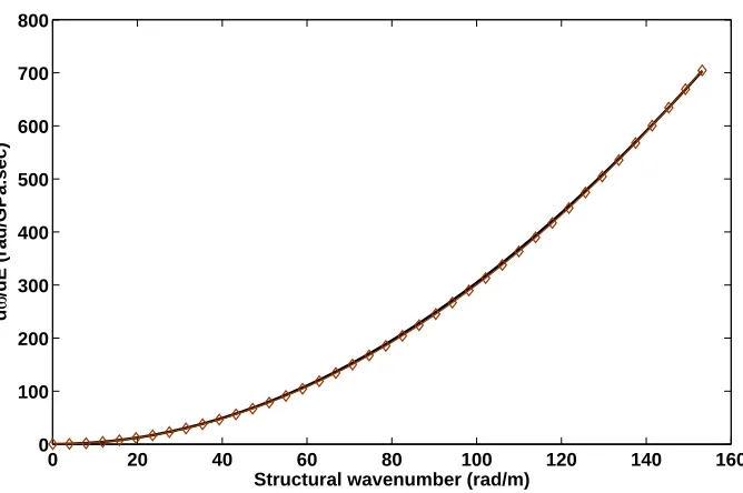
thickness. The first result in Fig.2 refers to the sensitivity of ω at which a

specific εx, εy set occurs for the first bending wave propagating in the

struc-ture. Real values are considered forεx, εy throughout this paper. The result

is compared to the CPT theory by differentiating the expression relating the

flexural wavenumber kf to the angular frequency ωf

ωf =

k2

f r

ρh Dm

(51)

with Dm =

Eh3

12(1−v2₎ the flexural stiffness of a monolayer panel. Very good agreement is observed between the two curves with the maximum divergence

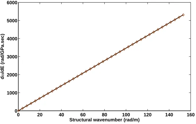
being equal to 0.18%. The perturbation of ω for the first membrane wave

propagating in the structure with relation toE is presented in Fig.3. The

re-sult is compared to the CPT theory by differentiating the expression relating

the membrane wavenumber km to the angular frequency ωm

ωm =

km r

ρ(1−v2₎ E

(52)

Again excellent agreement is observed between the analytical and

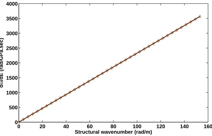
numeri-cal results. The perturbation of ω for the first shear wave propagating in

the structure with relation to E is presented in Fig.4. The result is

com-pared to the CPT theory by differentiating the expression relating the shear

wavenumber ks to the angular frequency ωs

ωs=

ks r

2ρ(1 +v) E

0 20 40 60 80 100 120 140 160 0

100 200 300 400 500 600 700 800

Structural wavenumber (rad/m)

d

ω

/dE (rad/GPa.sec)

0 20 40 60 80 100 120 140 160 0

1000 2000 3000 4000 5000 6000

Structural wavenumber (rad/m)

d

ω

/dE (rad/GPa.sec)

0 20 40 60 80 100 120 140 160 0

500 1000 1500 2000 2500 3000 3500 4000

Structural wavenumber (rad/m)

d

ω

/dE (rad/GPa.sec)

Figure 4: Sensitivity of the angular frequency ω at which the set of εx, εy occur under a perturbation of E for the first shear wave type: Analytical solution (⋄), Numerical calculation (−)

Again excellent correlation is observed between the analytical and numerical

results. As expected, throughout Fig.2-4 it is exhibited that an increase of

E would stiffen the structure, shifting a certain wavenumber value towards

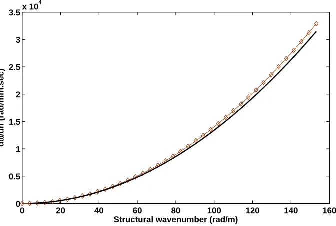
higher frequencies. The perturbation of ω for the first flexural wave

propa-gating in the structure with relation to the thickness h is presented in Fig.5.

Good agreement is generally observed between the results, however there is a

maximum discrepancy of 4.3% between the two curves. This is probably due

to an insufficiency of the analytical approach for modelling the dynamic

be-haviour at higher frequencies. Again an increase in thickness will stiffen the

structure, shifting the same wavenumber towards higher frequencies. There

0 20 40 60 80 100 120 140 160 0

0.5 1 1.5 2 2.5 3

3.5x 10

4

Structural wavenumber (rad/m)

d

ω

/dh (rad/mm.sec)

Figure 5: Sensitivity of the angular frequency ω at which the set ofεx,εy occur under a perturbation of the thickness of the structure for the first flexural wave type: Analytical solution (⋄), Numerical calculation (−)

structure, therefore the corresponding results are not presented for the sake

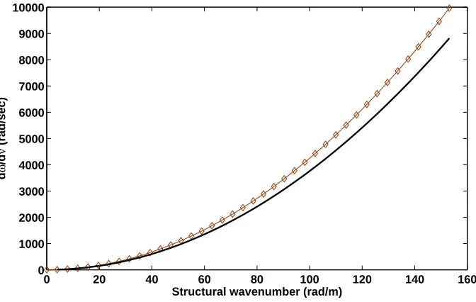
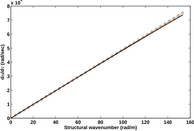
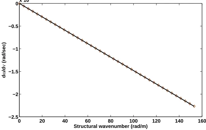
of brevity. The perturbation of ω with respect to the Poisson’s ratio of

the structure for the flexural, membrane and shear waves are presented in

Fig.6,7 and 8 respectively. A generally good agreement is observed between

the numerical and analytical results. Again for the flexural wave a

maxi-mum discrepancy of 11.5% between the two curves is taking place for high

wavenumber values due to the same aforementioned reason. It is interesting

to note that while increasing the Poisson’s ratio of the structure acts as a

stiffening effect for the flexural and membrane wave types, the same positive

perturbation ofv will result in shifting the shear wavenumber curves towards

0 20 40 60 80 100 120 140 160 0

1000 2000 3000 4000 5000 6000 7000 8000 9000 10000

Structural wavenumber (rad/m)

d

ω

/d

ν

(rad/sec)

0 20 40 60 80 100 120 140 160 0

1 2 3 4 5 6 7

8x 10

4

Structural wavenumber (rad/m)

d

ω

/d

ν

(rad/sec)

0 20 40 60 80 100 120 140 160 −2.5

−2 −1.5 −1 −0.5

0x 10

5

Structural wavenumber (rad/m)

d

ω

/d

ν

(rad/sec)

3.2. Sandwich panel

A sandwich panel comprising two facesheets and a core is modelled in

this section. The lower facesheet has a thickness hf l=0.001m and is made

of a material with ρf l=3000 kg/m3, Ef l = 70GPa and vf l=0.1. The upper

facesheet has a thickness equal to hf u=0.002m and is made of the same

material as the lower facesheet. The core has a thickness hc=0.01m and is

made of a material withρc=50 kg/m3,Ec = 0.07GPa andvc=0.4. Three FE

are used in the sense of thickness in order to model the structure. For the

sake of brevity and because of the fact that the out of plane waves are usually

the ones that are of interest for vibroacoustic, health monitoring and energy

harvesting applications -carrying most of the vibrational energy-, only results

on the flexural wave type are presented for the sandwich structure below. The

results are compared to a FD approach throughout this section. In order to

implement the FD approach a perturbation of 0.001% was considered for

each structural parameter. The resulting FD sensitivity can be computed by

∂ω ∂β =

ωp−ω0 βp−β0

(54)

with ωp the perturbated angular frequency at which a certain wavenumber

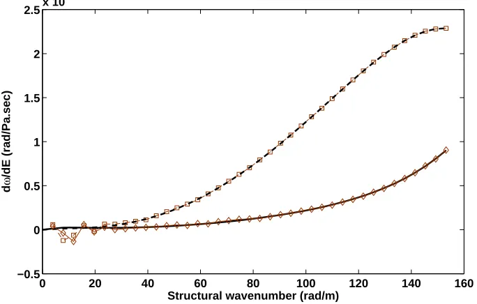
value occurs for βp and ω0 the corresponding angular frequency forβ0. The perturbation of ω with respect to Ef l, Ef u of the structure is presented in

Fig.9. It is observed that the increase of both values will stiffen the sandwich

structure. For the lower wavenumber values this increase in stiffness will

be similar for δEf l and δEf u. However in higher frequencies it can be seen

that increasing Ef u for the thicker upper facesheet will have a much greater

0 20 40 60 80 100 120 140 160 −0.5

0 0.5 1 1.5 2

2.5x 10

−7

Structural wavenumber (rad/m)

d

ω

/dE (rad/Pa.sec)

0 20 40 60 80 100 120 140 160 −2

0 2 4 6 8 10 12

14x 10

−5

Structural wavenumber (rad/m)

d

ω

/dE (rad/Pa.sec)

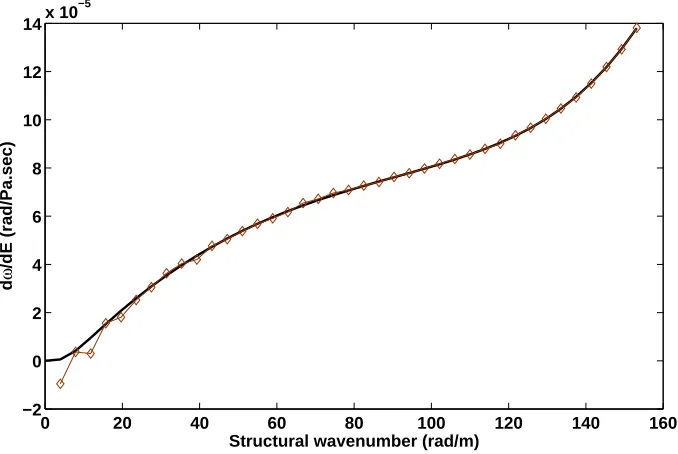
Figure 10: Sensitivity of the angular frequency ω at which the set of εx, εy occur under a perturbation of Ec for the first flexural wave type of a layered structure: Presented approach (−), FD computation (⋄)

ω with respect to Ec is presented in Fig.10. A fluctuation of the FD results

is observed again for low wavenumber values however the results are in very

good agreement for higher frequencies. Again it is observed that the effect

of δEc on the flexural wavenumber varies significantly with respect to the

wavenumber value. The perturbation of ω with respect to hf l, hf u of the

structure is presented in Fig.11. It is particularly interesting to note that for

lower wavenumbers increasing the thickness of both facesheets will imply a

softening effect to the structural behaviour, shifting the flexural wavenumbers

to lower frequencies. This mainly suggests that the effect of the added mass

overcomes the effect of added stiffness. This effect is similar for both δhf l

0 20 40 60 80 100 120 140 160 −2000

0 2000 4000 6000 8000 10000 12000 14000 16000 18000

Structural wavenumber (rad/m)

d

ω

/dh (rad/mm.sec)

Figure 11: Sensitivity of the angular frequencyω at which the set ofεx,εy occur under a perturbation of the thickness of the sandwich facesheets for the first flexural wave type of a layered structure: Presented approach forhf l(−), FD computation forhf l(⋄), Presented approach for hf u (−−), FD computation forhf u ()

change radically for the thicker upper facesheet, with δhf u now shifting the

wavenumbers to higher frequencies. Again excellent agreement is observed

between the presented approach and the FD method. The perturbation ofω

with respect to hc of the sandwich is presented in Fig.12. A very interesting

effect is that the influence of δhc on the flexural wavenumber becomes

max-imum at a certain wavenumber value (approximately for k=100rad/m). A

constant decrease of this influence is observed beyond that point. The

stiffen-ing effect is probably due to the greater separation of the two facesheets with

δhc. It is very probable however that for higher wavenumber values δhc will

have a softening effect on the flexural wavenumber with the depicted curve

0 20 40 60 80 100 120 140 160 0

50 100 150 200 250 300 350

Structural wavenumber (rad/m)

d

ω

/dh (rad/mm.sec)

0 20 40 60 80 100 120 140 160 0

1000 2000 3000 4000 5000 6000

Structural wavenumber (rad/m)

d

ω

/d

ν

(rad/sec)

Figure 13: Sensitivity of the angular frequency ω at which the set of εx, εy occur under a perturbation of the Poisson’s ratio of the sandwich facesheets for the first flexural wave type of a layered structure: Presented approach forvf l(−), FD computation forvf l (⋄), Presented approach forvf u(−−), FD computation forvf u ()

vf u of the structure is presented in Fig.13. In both cases it can be observed

that increasing v for the facesheets will shift the flexural wavenumber curve

towards higher frequencies. This phenomenon however will be much more

intense for δvf u especially at higher wavenumber values. Again excellent

agreement is observed between the FD results and the presented approach.

The perturbation of ω with respect to vc for the sandwich core is presented

in Fig.14. The effect of δvc is softening up to a certain wavenumber value,

beyond which a sudden exponential increase is observed which stiffens the

flexural structural behaviour. The perturbation of ω with respect to ρf l and

ρf u is presented in Fig.15. As expected both δρf l and δρf u will shift the

0 20 40 60 80 100 120 140 160 −5000

0 5000 10000 15000 20000

Structural wavenumber (rad/m)

d

ω

/d

ν

(rad/sec)

0 20 40 60 80 100 120 140 160 −6

−5 −4 −3 −2 −1 0

Structural wavenumber (rad/m)

d

ω

/d

ρ

(rad.m

3 /sec.kg)

Figure 15: Sensitivity of the angular frequency ω at which the set of εx, εy occur under a perturbation of the mass density of the sandwich facesheets for the first flexural wave type: Presented approach for ρf l (−), FD computation for ρf l (⋄), Presented approach forρf u (−−), FD computation forρf u()

thicker upper facesheet at low k values. It is very interesting however to

see that there is a critical wavenumber value (approximately k=147rad/m)

at which the effect of δρf l and δρf u will be the same. Beyond this critical

wavenumber the softening effect will be more intense forδρf l thanδρf u. The

perturbation of ω with respect to ρc for the sandwich core is presented in

Fig.16. It is clear that δρc implies a softening effect to the flexural behaviour

of the panel which has an increasing intensity with wavenumber values.

Throughout Fig.9-16, a great wavenumber dependence has been observed

for the sensitivity results of the sandwich structure. This exhibits the

0 20 40 60 80 100 120 140 160 −40

−35 −30 −25 −20 −15 −10 −5 0

Structural wavenumber (rad/m)

d

ω

/d

ρ

(rad.m

3 /sec.kg)

Figure 16: Sensitivity of the angular frequency ω at which the set of εx, εy occur un-der a perturbation of ρc for the first flexural wave type: Presented approach (−), FD computation (⋄)

layer for specific applications. The model can also be used for computing

the effect of the inclusion of smart layers such as auxetics and piezoelectrics

or computing the sensitivity of the propagating waves in the presence of

damage.

4. Conclusions

A numerical continuum-discrete approach for computing the sensitivity

of the waves propagating in periodic structures was presented in this paper.

The main conclusions of the work are as follows:

(i) A formulation of the two dimensional wave propagation problem was

propagating in the periodic structure. The structure can be of arbitrary

layering, material characteristics and geometric complexity. The effect of

local parameter variation can also be considered.

(ii) A reduced transfer matrix formulation of the wave propagation

anal-ysis in one dimensional periodic media was presented, followed by the

deriva-tion of the sensitivity of the wavenumber values. As for the first formuladeriva-tion,

the structure can be of arbitrary layering, material characteristics and

geo-metric complexity. This approach however tends to be less computationally

efficient due to the involved inversions and multiplications of DSM partitions.

(iii) A monolayer panel was modelled by the presented approach and the

resulting sensitivity values were validated through the CPT.

(iv) Moreover, an asymmetric sandwich structure was also modelled. The

sensitivity of the propagating flexural wave with respect to the structural

parameters of the facesheets and the core were computed and the results

were successfully compared to the ones provided by the FD method.

(v) A great wavenumber dependence has been observed for the sensitivity

results of the sandwich structure. This exhibits the potential of the presented

tool with regard to providing an efficient and robust optimization scheme for

layered structures, tailored for specific applications. The model can also be

used for computing the effect of the inclusion of smart layers such as auxetics

and piezoelectrics or computing the sensitivity of the propagating waves in

the presence of damage.

(vi) The formulation of the symbolic expression of the stiffness and mass

matrices for a linear solid FE were also presented. These formulations can

modelled segment, as well as the sensitivity of the global matrices with regard

to any structural parameter.

References

[1] D. J. Mead, A general theory of harmonic wave propagation in linear

periodic systems with multiple coupling, Journal of Sound and Vibration

27 (1973) 235–60.

[2] R. Langley, A note on the force boundary conditions for two-dimensional

periodic structures with corner freedoms, Journal of Sound and

Vibra-tion 167 (1993) 377–81.

[3] W. Zhong, F. Williams, On the direct solution of wave propagation

for repetitive structures, Journal of Sound and Vibration 181 (1995)

485–501.

[4] B. R. Mace, D. Duhamel, M. J. Brennan, L. Hinke, Finite element

prediction of wave motion in structural waveguides, The Journal of the

Acoustical Society of America 117 (2005) 2835–43.

[5] J.-M. Mencik, M. Ichchou, Multi-mode propagation and diffusion in

structures through finite elements, European Journal of

Mechanics-A/Solids 24 (2005) 877–98.

[6] D. Duhamel, B. R. Mace, M. J. Brennan, Finite element analysis of the

vibrations of waveguides and periodic structures, Journal of Sound and

[7] J.-M. Mencik, On the low-and mid-frequency forced response of elastic

structures using wave finite elements with one-dimensional propagation,

Computers & Structures 88 (2010) 674–89.

[8] J. M. Renno, B. R. Mace, On the forced response of waveguides using

the wave and finite element method, Journal of Sound and Vibration

329 (2010) 5474–88.

[9] B. Mace, E. Manconi, Modelling wave propagation in two-dimensional

structures using finite element analysis, Journal of Sound and Vibration

318 (2008) 884–902.

[10] J. Renno, B. Mace, Calculating the forced response of two-dimensional

homogeneous media using the wave and finite element method, Journal

of Sound and Vibration 330 (2011) 5913–27.

[11] D. Chronopoulos, B. Troclet, M. Ichchou, J. Laine, A unified approach

for the broadband vibroacoustic response of composite shells,

Compos-ites Part B: Engineering 43 (2012) 1837–46.

[12] D. Chronopoulos, B. Troclet, O. Bareille, M. Ichchou, Modeling the

re-sponse of composite panels by a dynamic stiffness approach, Composite

Structures 96 (2013) 111–20.

[13] D. Chronopoulos, M. Ichchou, B. Troclet, O. Bareille, Efficient

predic-tion of the response of layered shells by a dynamic stiffness approach,

Composite Structures 97 (2013) 401–4.

[14] D. Chronopoulos, M. Ichchou, B. Troclet, O. Bareille, Predicting the

loads by a krylov subspace reduction, Applied Acoustics 74 (2013) 1394–

405.

[15] D. Chronopoulos, M. Ichchou, B. Troclet, O. Bareille, Thermal

ef-fects on the sound transmission through aerospace composite structures,

Aerospace Science and Technology 30 (2013) 192–9.

[16] D. Chronopoulos, M. Ichchou, B. Troclet, O. Bareille, Predicting the

broadband response of a layered cone-cylinder-cone shell, Composite

Structures 107 (2014) 149–59.

[17] D. Chronopoulos, M. Ichchou, B. Troclet, O. Bareille, Computing the

broadband vibroacoustic response of arbitrarily thick layered panels by

a wave finite element approach, Applied Acoustics 77 (2014) 89–98.

[18] V. Polenta, S. Garvey, D. Chronopoulos, A. Long, H. Morvan, Optimal

internal pressurisation of cylindrical shells for maximising their critical

bending load, Thin-Walled Structures 87 (2015) 133–8.

[19] T. Ampatzidis, D. Chronopoulos, Acoustic transmission properties of

pressurised and pre-stressed composite structures, Composite Structures

152 (2016) 900–12.

[20] I. Antoniadis, D. Chronopoulos, V. Spitas, D. Koulocheris,

Hyper-damping properties of a stiff and stable linear oscillator with a negative

stiffness element, Journal of Sound and Vibration 346 (2015) 37–52.

[21] D. Chronopoulos, M. Collet, M. Ichchou, Damping enhancement of

composite panels by inclusion of shunted piezoelectric patches: A

[22] D. Chronopoulos, I. Antoniadis, M. Collet, M. Ichchou, Enhancement of

wave damping within metamaterials having embedded negative stiffness

inclusions, Wave Motion 58 (2015) 165–79.

[23] D. Chronopoulos, Design optimization of composite structures operating

in acoustic environments, Journal of Sound and Vibration 355 (2015)

322–44.

[24] M. Ben Souf, D. Chronopoulos, M. Ichchou, O. Bareille, M. Haddar,

On the variability of the sound transmission loss of composite panels

through a parametric probabilistic approach, Journal of Computational

Acoustics 24 (2016).

[25] D. Chronopoulos, Wave steering effects in anisotropic composite

struc-tures: Direct calculation of the energy skew angle through a finite

ele-ment scheme, Ultrasonics 73 (2017) 43–8.

[26] R. B. Nelson, Simplified calculation of eigenvector derivatives, AIAA

journal 14 (1976) 1201–5.

[27] R. T. Haftka, H. M. Adelman, Recent developments in structural

sen-sitivity analysis, Structural optimization 1 (1989) 137–51.

[28] S. Adhikari, M. I. Friswell, Eigenderivative analysis of asymmetric

non-conservative systems, International Journal for Numerical Methods in

Engineering 51 (2001) 709–33.

[29] K. K. Choi, N.-H. Kim, Structural sensitivity analysis and optimization

[30] K. Sobczyk, Stochastic wave propagation, Elsevier, 1985.

[31] A. Belyaev, Comparative study of various approaches to stochastic

elas-tic wave propagation, Acta mechanica 125 (1997) 3–16.

[32] K. Koo, B. Pluymers, W. Desmet, S. Wang, Vibro-acoustic design

sen-sitivity analysis using the wave-based method, Journal of Sound and

Vibration 330 (2011) 4340–51.

[33] M. Ruzzene, F. Scarpa, Directional and band-gap behavior of periodic

auxetic lattices, physica status solidi (b) 242 (2005) 665–80.

[34] M. Ichchou, F. Bouchoucha, M. Ben Souf, O. Dessombz, M. Haddar,

Stochastic wave finite element for random periodic media through

first-order perturbation, Computer Methods in Applied Mechanics and

En-gineering 200 (2011) 2805–13.

[35] B. Souf, O. Bareille, M. Ichchou, F. Bouchoucha, M. Haddar, Waves

and energy in random elastic guided media through the stochastic wave

finite element method, Physics Letters A 377 (2013) 2255–64.

[36] V. Cotoni, R. S. Langley, P. J. Shorter, A statistical energy analysis

sub-system formulation using finite element and periodic structure theory,

Journal of Sound and Vibration 318 (2008) 1077–108.

[37] S. Finnveden, Evaluation of modal density and group velocity by a finite

element method, Journal of Sound and Vibration 273 (2004) 51–75.

[38] C. A. Felippa, R. W. Clough, The finite element method in solid

X

Y

Z

L

_x

L

_y

L

_z

Figure 17: The considered solid FE

Appendix A. Sensitivity analysis of a solid FE

A linear solid FE is hereby considered as shown in Fig.17. Following

described as          x y z          =     

x1 x2 x3 x4 x5 x6 x7 x8

y1 y2 y3 y4 y5 y6 y7 y8

z1 z2 z3 z4 z5 z6 z7 z8

                                            N1 N2 N3 N4 N5 N6 N7 N8                                        (A.1)

The displacement interpolations are expressed as

         ux uy uz          =     

ux1 ux2 ux3 ux4 ux5 ux6 ux7 ux8 uy1 uy2 uy3 uy4 uy5 uy6 uy7 uy8 uz1 uz2 uz3 uz4 uz5 uz6 uz7 uz8

Linear shape functions are assumed for the element

N1 = 1₈(1−ξ)(1−η)(1 +µ)

N2 = 1₈(1−ξ)(1−η)(1−µ)

N3 = 1₈(1−ξ)(1 +η)(1−µ)

N4 = 1₈(1−ξ)(1 +η)(1 +µ)

N5 = 1₈(1 +ξ)(1−η)(1 +µ)

N6 = 1₈(1 +ξ)(1−η)(1−µ)

N7 = 1₈(1 +ξ)(1 +η)(1−µ)

N8 = 1₈(1 +ξ)(1 +η)(1 +µ)

(A.3)

The element stiffness matrix k is formally given by the volume integral

k= Z 1

−1

Z 1

−1

Z 1

−1

B⊤_{DB|J|dηdξdµ (A.4)}

while the element mass matrix m can be determined as

m= Z 1

−1

Z 1

−1

Z 1

−1

N⊤_{ρmN|J| dηdξdµ (A.5)}

with

N= 

   

N1 0 0 · · · N8 0 0

0 N1 0 · · · 0 N8 0

0 0 N1 · · · 0 0 N8



   

while ρm is the mass density of the material. It is also noted that B =               ∂N1

∂x 0 0

∂N2

∂x · · ·

∂N8

∂x 0 0

0 ∂N1

∂y 0 0 · · · 0

∂N8

∂y 0

0 0 ∂N1

∂z 0 · · · 0 0

∂N8 ∂z ∂N1 ∂y ∂N1 ∂x 0 ∂N2

∂y · · ·

∂N8

∂y ∂N8

∂x 0

0 ∂N1

∂z ∂N1

∂y 0 · · · 0

∂N8 ∂z ∂N8 ∂y ∂N1 ∂z 0 ∂N1 ∂x ∂N2

∂z · · ·

∂N8 ∂z 0 ∂N8 ∂x                                                     

ux1 uy1 uz1 ux2

· · ·

ux8 uy8 uz8

                                       (A.7)

The Jacobian matrix of the element is

J=        ∂x ∂ξ ∂y ∂ξ ∂z ∂ξ ∂x ∂η ∂y ∂η ∂z ∂η ∂x ∂µ ∂y ∂µ ∂z ∂µ        (A.8)

while the the flexibility matrix of the element for an orthotropic material

D−1 _{can generally be written as}

D−1 ₌

                  1 Ex

−vxy

Ex

−vxz

Ex

0 0 0

−vyx

Ey

1 Ey

−vyz

Ey

0 0 0

−vzx

Ez

−vzy

Ez

1 Ez

0 0 0

0 0 0 1

Gxy

0 0

0 0 0 0 1

Gyz

0

0 0 0 0 0 1

Gxz                   (A.9)

The assumption of the undeformed FE being a rectangular parallelepiped is

andz1, z2, z3, z4, z5, z6, z7, z8,can then be replaced byLx, Ly, Lz in the

expres-sion of B. The generic expression form is thus given as

m= (ρLxLyLz)

                                                                   

1/27 0 0 1/54 0 0 1/108 0 0 1/54 0 0 1/54 0 0 1/108 0 0 1/216 0 0 1/108 0 0

0 1/27 0 0 1/54 0 0 1/108 0 0 1/54 0 0 1/54 0 0 1/108 0 0 1/216 0 0 1/108 0

0 0 1/27 0 0 1/54 0 0 1/108 0 0 1/54 0 0 1/54 0 0 1/108 0 0 1/216 0 0 1/108

1/54 0 0 1/27 0 0 1/54 0 0 1/108 0 0 1/108 0 0 1/54 0 0 1/108 0 0 1/216 0 0

0 1/54 0 0 1/27 0 0 1/54 0 0 1/108 0 0 1/108 0 0 1/54 0 0 1/108 0 0 1/216 0

0 0 1/54 0 0 1/27 0 0 1/54 0 0 1/108 0 0 1/108 0 0 1/54 0 0 1/108 0 0 1/216

1/108 0 0 1/54 0 0 1/27 0 0 1/54 0 0 1/216 0 0 1/108 0 0 1/54 0 0 1/108 0 0

0 1/108 0 0 1/54 0 0 1/27 0 0 1/54 0 0 1/216 0 0 1/108 0 0 1/54 0 0 1/108 0

0 0 1/108 0 0 1/54 0 0 1/27 0 0 1/54 0 0 1/216 0 0 1/108 0 0 1/54 0 0 1/108

1/54 0 0 1/108 0 0 1/54 0 0 1/27 0 0 1/108 0 0 1/216 0 0 1/108 0 0 1/54 0 0

0 1/54 0 0 1/108 0 0 1/54 0 0 1/27 0 0 1/108 0 0 1/216 0 0 1/108 0 0 1/54 0

0 0 1/54 0 0 1/108 0 0 1/54 0 0 1/27 0 0 1/108 0 0 1/216 0 0 1/108 0 0 1/54

1/54 0 0 1/108 0 0 1/216 0 0 1/108 0 0 1/27 0 0 1/54 0 0 1/108 0 0 1/54 0 0

0 1/54 0 0 1/108 0 0 1/216 0 0 1/108 0 0 1/27 0 0 1/54 0 0 1/108 0 0 1/54 0

0 0 1/54 0 0 1/108 0 0 1/216 0 0 1/108 0 0 1/27 0 0 1/54 0 0 1/108 0 0 1/54

1/108 0 0 1/54 0 0 1/108 0 0 1/216 0 0 1/54 0 0 1/27 0 0 1/54 0 0 1/108 0 0

0 1/108 0 0 1/54 0 0 1/108 0 0 1/216 0 0 1/54 0 0 1/27 0 0 1/54 0 0 1/108 0

0 0 1/108 0 0 1/54 0 0 1/108 0 0 1/216 0 0 1/54 0 0 1/27 0 0 1/54 0 0 1/108

1/216 0 0 1/108 0 0 1/54 0 0 1/108 0 0 1/108 0 0 1/54 0 0 1/27 0 0 1/54 0 0

0 1/216 0 0 1/108 0 0 1/54 0 0 1/108 0 0 1/108 0 0 1/54 0 0 1/27 0 0 1/54 0

0 0 1/216 0 0 1/108 0 0 1/54 0 0 1/108 0 0 1/108 0 0 1/54 0 0 1/27 0 0 1/54

1/108 0 0 1/216 0 0 1/108 0 0 1/54 0 0 1/54 0 0 1/108 0 0 1/54 0 0 1/27 0 0

0 1/108 0 0 1/216 0 0 1/108 0 0 1/54 0 0 1/54 0 0 1/108 0 0 1/54 0 0 1/27 0

0 0 1/108 0 0 1/216 0 0 1/108 0 0 1/54 0 0 1/54 0 0 1/108 0 0 1/54 0 0 1/27

                                                                    (A.10)

while the symbolic generic expression ofkcan be derived exactly in the same way but is hereby intentionally omitted for the sake of brevity.

The generic sensitivity expressions ∂k ∂βi

, ∂m ∂βi

as well as ∂ 2_k ∂βj∂βi

, ∂ 2_m ∂βj∂βi

with βi, βj being design parameters can therefore be calculated as a function

of Ex, Ey, Ez, vxy, vxz, vyz,Gxy, Gxz, Gyz, Lx, Ly, Lz by differentiating over the

List of symbols

ℜ Real operator

D Dynamics Stiffness Matrix (DSM) of a waveguide’s modelled periodic segmen M, K Mass and stiffness matrices of the modelled segment

T Wave propagation transfer matrix

R Transformation matrix

m, k Mass and stiffness matrices of a single FE

f Forcing vector for an elastic waveguide

q Physical displacement vector for an elastic waveguide

x Reduced set of DoF

x0i Unperturbed eigenvector of the DSM

y0i Unperturbed left eigenvector of wave transfer matrixT z0i Unperturbed right eigenvector of wave transfer matrix T

B,T, L,R, I Bottom, Top, Left, Right sides and Internal indices

E Material Young’s modulus

Lx, Ly Dimensions of the entire panel

h Thickness

k Wavenumber

lx,ly Dimensions of the modelled periodic structural segment

s Periodic segment positioning index

t Time

x, y Propagation directions

β Design variable

γ Propagation constant and eigenvalue of wave transfer matrixT

ǫ Perturbation coefficient

ε Propagation constant

λ Eigenvalue of the DSM

v Poisson’s ratio

ρ Material density

List of abbreviations

CPT Classical Plate Theory

DoF Degree of Freedom

DSM Dynamic Stiffness Matrix

FD Finite Differences

FE Finite Element

PST Periodic Structure Theory