Urban VANET performance optimization

(1)

University of Warwick institutional repository:

http://go.warwick.ac.uk/wrap

A Thesis Submitted for the Degree of PhD at the University of Warwick

http://go.warwick.ac.uk/wrap/63931

This thesis is made available online and is protected by original copyright.

Please scroll down to view the document itself.

(2)

Urban VANET

Performance Optimization

by

Xiang Yu

A dissertation submitted in fulfillment of the

Requirements for the degree of Doctor of Philosophy

University of Warwick, School of Engineering

(3)

Foreword

Acknowledgements………..…i

Declaration…………..………ii

Abstract………iii

List of Figures………..………v

List of Tables……….viii

Acknowledgements

I would like to take this opportunity to thank my supervisors, Dr. Mark Leeson

and Prof. Evor Hines, for their academic support, supervision during my Ph.D

stage, and motivation whenever I was depressed. Without their contributions

this work will never come to a reality.

I would also like to thank my colleagues working with me in A405a lab, your

academic excellence and inspirational spirit always encouraged me. The group discussion and your valuable feedback to my project benefit me a lot. Wish you

all have a splendid future.

Special thanks here to my family: my dad and mum who sponsored me in this

project, my wife Sue always supported me when I was in difficulties and depression. Without your encouragement I will never finish this thesis.

Last but not least, thanks to all academic staff who discussed with me about my

(6)

ii

Declaration

The work described in this thesis was conducted by the author, except where stated otherwise, in the School of Engineering, University of Warwick between

the dates of March 2010 and December 2013. No part of this work has been previously submitted to the University of Warwick or any other academic

institution for admission to a higher degree. All publications to date arising

(7)

iii

Abstract

Urban VANET (Vehicular Ad hoc NETworks) performance optimization

concerns the improvement of wireless signal quality between two arbitrary

selected nodes moving within along city streets. It includes three procedures:

VANET architecture modeling; wireless signal simulation; and signal quality optimization techniques. The first procedure converts real-world map data into

a network graph according to the requirement of the optimization algorithm.

The second step analyzes a communication route between two network nodes and calculates received signal quality with the information provided by the

network model. The final operation optimizes the signal quality to an expected

level by choosing appropriate communication route between two wireless

nodes.

In this thesis, three optimization techniques are presented: EP (Evolutionary

Programming), SG (Stochastic Geometry) and SW (Small World). EP is a widely

applied optimization strategy based on Darwin’s natural selection and evolution theory. It is effective with an enormous number of data support, and

it can provide detailed route information. However, it requires enough time to

evolve to an optimal solution. SG is a statistical tool to analyze points’ distribution within a multi-dimensional space, and it was recently applied on

wireless network analysis. Given the distribution characteristics of an urban

area, SG can calculate average data loss rate of a communication route. However, it cannot provide detailed route information. SW is a widely accepted

(8)

iv

in VANET analysis. SW provides a simplified network architecture compared

with EP an SG. However, it requests additional long-range communication equipment and consumes more energy.

The thesis is divided into three parts. Chapter 1 introduces the history of

VANET and its architecture (in this research, it is a combination of Ad hoc network and WSN (Wireless Sensor Network). Chapter 2 and 3 presents

literature review of EP and SG. Chapter 4, 5, and 6 discusses how to implement

(9)

v

List of Figures

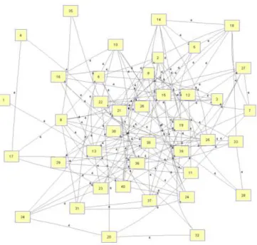
Fig. 1.1 A 40-node Ad hoc network frame (created by Gaussian distribution) --4

Fig. 1.2 A sample WSN diagram in urban area---10

Fig. 2.1 European Cost239 Network—Topology with actual distances in km--25

Fig. 2.2 Example of dynamic connection requests ---27

Fig. 2.3: Example of alternative path selection ---28

Fig. 2.4 Flow chart of genetic algorithm process ---30

Fig. 2.5: Crossover operation ---33

Fig. 2.6 Mutation operation---34

Fig. 2.7 AWUT optimization result ---35

Fig. 2.8 ALR result for 8 iterations ---37

Fig. 2.9 TBP optimization result after 8 iterations ---39

Fig. 2.10 Random 40-node network ---40

Fig. 3.1. (a) A 4040 km view of a current base station deployment by a major service provider in a relatively flat urban area; (b) a Poisson distributed base stations, with each mobile associated with the nearest base station ---52

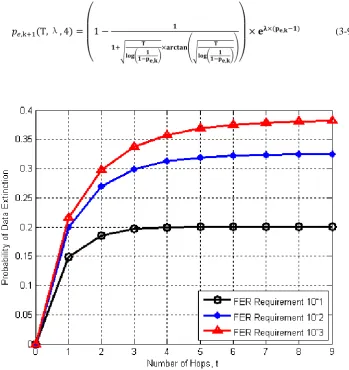
Fig. 3.2 Diagram of multi-hops and probability of data extinction ---55

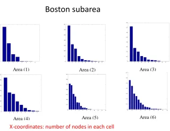
Fig. 3.3. Area division of Boston city ---56

Fig. 3.4.Probability density distributions (PDF) of 6 areas ---57

(10)

vi

Fig. 4.1 (a) Triangle formation; (b) Boston repeater network ---64

Fig. 4.2 Two PDF bar graphs from Boston city streets ---65

Fig. 4.3 Triangle map formation: (a) urban zones; (b) triangle formation ---67

Fig. 4.4 Data structure of Boston city streets ---71

Fig. 4.5 Labeling street zones of Boston city center ---72

Fig. 4.6 Static connection requests ---74

Fig. 4.7 Dynamic source flow chart ---77

Fig. 4.9 Search space, initial populations, optimal Pareto set ---82

Fig. 4.10 Optimization factor space—single objective optimization ---84

Fig. 4.11 Optimization factor space—multiple objective optimizations ---85

Fig. 5.1 Boston street junctions—7 sub areas ---91

Fig. 5.2 node distributions of 6 Boston city subareas ---93

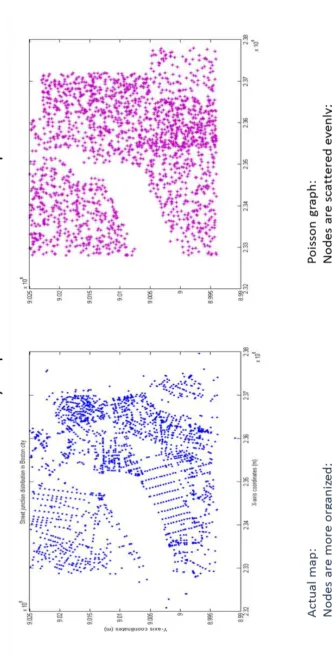
Fig. 5.3 Boston city map versus Poisson virtual map ---96

Fig. 5.4 PDF of Data Extension (theoretical) ---97

Fig. 5.5 Markov Chain State Flow Graph of the Boston city ---98

Fig. 5.6 Data loss rate curves on 6 Boston subareas ---101

Fig. 5.7 Simulation results of EP (above) and SG (down) ---105

Fig. 6.1 Small world effect diagrams ---110

(11)

vii

Fig. 6.3 Powerful sensor placement diagram ---116

Fig. 6.4 Small-world connection (re-wiring probability β= 0.01) ---116

Fig. 6.5 Small-world connection (re-wiring probability β = 0.1) ---117

Fig. 6.6 Small-world connection (re-wiring probability β = 0.6) ---117

Fig. 6.7 Curve of BER (in red) and Energy (in blue) versus Re-wiring probability---120

Fig. 6.8 Signal quality efficiency versus re-wiring probability β---122

Fig. 7.1 OFDM block diagram ---127

Fig. 7.2 Probability of correct detection of the paths in OFDM scenario---128

Fig. 7.3 Dual antenna WAVE block diagram ---129

(12)

viii

List of tables

Table 1.1 Characteristics of source initiated ad hoc routing protocols---7

Table 1.2 Impact Factor of TVT---13

Table 2.1 Example of scheduled traffic requests---26

Table 2.2: Available links of each node in Cost 239 network ---27

Table 2.3: Example of Path Set Series---28

Table 2.4 Example of chromosome encoding---30

Table 2.5 Comparison of FF, DRCL and GA using four wavelengths and uniformly distributed traffic---41

Table 2.6 Comparison between FF and GA using 64 wavelengths and uniform traffic ---43

Table 2.7 Comparison between FF and GA using 64 wavelengths and randomly distributed traffic---44

Table 3.1 EP versus SG---50

Table 3.2 Values of Poisson model λ in seven subareas ---57

Table 3.3 Categories of city scenarios for stochastic geometry applications---60

Table 4.1 Inner-triangle data entry---67

Table 4.2 Inter-triangle data entry---69

Table 4.3 Sensor number matrix---70

Table 4.4 Initial population: 4 chromosomes---74

(13)

ix

Table 4.6 new populations from crossover operation---76

Table 4.7 Fitness values for initial population---77

Table 4.8 Primary and secondary population’s evolutions---79

Table 4.9 Computational complexity of the SRA algorithm---80

Table 5.1 Boston subarea information ---92

Table 5.2 Values of Poisson model λ in seven subareas---93

Table 5.3 Markov Chain transmit matrix values---100

Table 6.1 Simulation results of three small-world network scenarios---118

(14)

1

CHAPTER 1 V E H I C U L A R A D H O C N E T W O R K S

In this chapter a general overview is presented of VANETs (Vehicular Ad hoc NETworks), the domain in which this research was carried out. An

introduction of the origin of the VANET—wireless network (history, technical

breakthrough, current status) is firstly given. Then follows a brief review of two widely studied models in this field: ad hoc networks, and wireless sensor

networks, especially focusing on their network routing protocols. Since the

VANET model that has been applied in this research consists of ad hoc network node pairs and wireless sensor routers, the design of a routing protocol needs

to consider both of the networks’ characteristics. Finally a brief of key

conferences and organizations studying VANET is presented.

1.1 INTRODUCTION TO WIRELESS NETWORKS [1.1]

The use of wireless signals (signals whose frequencies are within the range 9

kHz to 300 GHz) in telecommunications can be dated back to the 1940s, when in the Second World War radio waves were applied for military purposes.

However, this technology was sealed within laboratories until long after the

war. At the beginning of the 1950s, Bell Labs in the United States deployed the first generation of wireless networks called the AMPS [1.2] (Advanced Mobile

Phone Service) network. Then it was standardized and commercialized in

North America in 1982. An AMPS network operated at a central frequency of

(15)

2

transferring analog signals. From then on, the evolution of wireless networks

has never ceased.

Until this very day, it has experienced four generations with a family of many

different standardized versions deployed in different areas. The latest wireless

network, branded as LTE [1.3] (Long Term Evolution) operates on various frequency bands (700, 800, 1900 and 1700/2100 MHz in North America;

2500 MHz in South America; 800, 900, 1800, 2600 MHz in Europe; 1800 and

2600 MHz in Asia; and 1800 MHz in Australia and New Zealand), supporting peak download rates of 300 Mbps and upload rates of 75.4 Mbps. Its channels

are transferring digital signals coded with vast many multimedia standards

(for example: JPEG for image compression, MPEG 2000 for video compression,

and AAC-ELD, Advanced Audio Coding for Enhanced Latency Delay). In addition, current wireless networks are not only interfacing with the PSTN

(Public Switched Telephone Network), but also interoperating with the

Internet, providing IP-based services [1.4]. From its physical infrastructure to virtual routing protocols, wireless networking is evolving more as an all IP

network, in common with the Internet. Many Internet based techniques can be

seamlessly applied on wireless networks, with only minor modifications to physical settings.

In the past decade, wireless networks have been studied by many researchers

due to their widespread application in daily life. However, much of the work

has been carried out in the free-space environment and assumed that signal propagation follows a simple line of sight (LOS) transmission model [1.5], [1.6].

There was thus a dearth of research were executed in the real urban area

(16)

3

across concrete walls before reaching their destinations. This situation lasted

until the last decade, when a transportation based system, the vehicular ad-hoc Network (VANET) was introduced and investigated in several industrial

projects [1.7], [1.8], [1.9]. As described in the subsequent reports and surveys,

a VANET is a mobile ad-hoc network (MANET), where vehicles act as nodes which are restricted to move along city streets[1.10], [1.11]. The VANET is

clearly a more realistic modeling of urban ad-hoc networks.

This research explores the possibility of communications on one and more pairs of VANET nodes through a sensor network. The signals originate and

terminate both on VANET nodes, which are restricted in an urban access area

(streets). However, these signals are forwarded through many sensor routers

before reaching their destinations. Many types of routing protocols exist in MANETs and wireless sensor networks (WSNs), and here these are reviewed

before the creation of a new strategy and its optimization. In section 1.2 and

1.3, these two types of wireless networks and their routing protocols are introduced. In section 1.4, an introduction to current mainstream international

conferences and journals is presented.

1.2 INTRODUCTION TO AD HOC NETWORKS [1.12]

Ad-hoc, itself a Latin phrase meaning ‘to this’. When used as a scientific term, it

generally specifies an object whose nature is flexible or unpredictable. As a member of the wireless network family, ad-hoc networks or MANETs, were

firstly introduced in the 1970s. The ALOHA network [1.13] which was carried

at University of Hawaii and sponsored by DARPA (Defense Advanced Research

(17)

4

802.11 [1.14], standardized and released at 1997 by the IET. A brief review has

been given to ad-hoc routing protocols which are directly associated with the research carried in this project. Chapter 4 further analyzes typical routing

[image:17.595.139.518.199.584.2]

protocols in ad-hoc networks.

Fig. 1.1 A 40-node ad-hoc network frame

(created by Matlab Gaussian distribution function)

(18)

5

a network is to use the Random Way Point model, which can be simulated

using a Matlab reference design [1.32].

According to [1.15], existing ad-hoc network routing protocols can be broadly

classified into as two types:

1. Table driven 2. Source initiated

In table-driven routing protocols, ad-hoc network information is stored in

routing tables maintained separately by its node members. This information may be their distances to a sourcing node, a cost defined by a specific protocol,

or anything useful in a network routing algorithm. Any changes to this

information will be broadcast within the whole network, and routing tables

will be updated accordingly. A routing enquiry from one node to another is transformed into a search of its routing table information. The protocol will

firstly seek for a direct match in its routing table, and no entry is found, seek

for an intermediate node (called a hop) to receive this enquiry. The table-driven routing technique was firstly used on the Internet, where equipment

(routers) is specially designed to maintain a table on all IP requests flowing

through it and direct different requests to their destinations according to its table recordings. Later on it was successfully applied on wireless ad-hoc

networks. However, as the fast-changing nature of an ad-hoc network, routing

information could expire in a shorter period, making it very difficult to be

precise.

(19)

6

a. Destination-Sequenced Distance-Vector Routing [1.16]

b. Cluster head Gateway Switch Routing [1.17] c. Wireless Routing Protocol [1.18]

Differently to the table-driven routing technique, source-initiated on-demand

routing is a reactive process only responding to source node requests. When a node in wireless network requires a communication to another node, it

initiates a connection request to the protocol. The protocol will then discover a

route for it and maintain this route until the communication is over.

a) Ad hoc On-Demand Distance Vector Routing [1.19]

b) Dynamic Source Routing [1.20]

c) Temporarily Ordered Routing Algorithm [1.21]

d) Associability-Based Routing [1.22] e) Signal Stability Routing [1.23]

These routing protocols share common characteristics, as are shown in table

1.1 [1.15]: they all target on flat network architecture; they are loop-free so they can avoid dead lock in a routing search; most of them are unicast, and

store their routing information in routing tables; many of them are using the

shortest path algorithm to look for the next hop. In conclusion, these routing protocols are very similar, so AODV is chosen to represent this

(20)

7

Table 1.1 Characteristics of source initiated ad hoc routing protocols [1.15]

Performance parameters AODV DSR TORA ABR SSR

Time complexity (initial) O(2d) O(2d) O(2d) O(d+z) O(d+z)

Time complexity (recover) O(2d) O(2d) O(2d) O(l+z) O(l+z)

Communication (initial) O(2N) O(2N) O(N+y) O(N+y) O(N+y)

Communication (failure) O(2N) O(2N) O(2x) O(x+y) O(x+y)

Routing philosophy Flat Flat Flat Flat Flat

Multicast capability Yes No No No No

Beaconing requests No No No Yes Yes

Multiple routing capabilities No Yes Yes No No

Routing maintained in Route table Route table Table Table Table

Route cache/expiration timers Yes No No No No

Route reconfiguration Erase route; notify source

notify source

Link reversal

broadcast query

notify source

Abbreviations:

l = diameter of the network; y = total number of nodes forming the directed path where

the REPLY packet transits; z = Diameter of the directed path where the REPLY packet

(21)

8

Current challenges for ad-hoc network routing protocols include:

 Multicast capabilities

 QoS in highly dynamic scenario

 Network security

 Interoperability with other types of networks (INTENET, Sensor

networks, etc)

To develop and maintain a multicast routing structure is very difficult for an

ad-hoc network because the multicast tree is no longer static. A dynamic routing strategy was mentioned in [1.24] to cope with dynamic multicast

decisions (for example, routing reestablishment strategies when nodes join or

leave the tree). How to maintain a stable, primary set of active connections under a highly dynamic environment needs to be considered by researchers.

Another important issue to solve is the Quality of Service (QoS) to improve end

user experience. Different level of customer needs brings different QoS demands of each active connection, and when a customer needs upgrades, the

routing protocol needs to allocate (reserve) enough network resources to

satisfy it. This kind of reservation may lead to a level of network redundancy, and a well-designed routing protocol shall locate a balance point between

redundancy and efficiency.

Finally, more and more researchers now focus on interoperability between ad-hoc networks and other types of networks. In this research, the possibility of

transmitting ad hoc signals through a sensor network is also explored. As is

shown in later sections, pre-deployed sensor networks can reduce

(22)

9

it may bring higher delay due to an enormous number of hops, it is still a

candidate for backup connections. A review of WSNs is given in the next section.

1.3 INTRODUCTION TO WIRELESS SENSOR NETWORKS

In contrast to the ad hoc network infrastructure, a WSN contains many more

nodes (hundreds, often thousands), but these sensors are lacking mobility,

with limited power supply, and can only perform very few communication tasks. In [18] the routing protocols are roughly classified into three types:

i. Flat

ii. Hierarchical iii. Location-based

Also these routing techniques can be divided into five categories according to

the routing information they use:

a. Multipath-based

b. Query-based

c. Negotiation-based

d. QOS (Quality of Service)-based e. Coherent-based

Many of routing protocols applied on WSNs are designed to save energy, which is a major concern in this network supplied with limited power resources.

However, the third category: location based routing protocols, is the key part

(23)

10

A mandate for a WSN to operate a location based routing protocol is to have its

sensor nodes GPS (Global Positioning System) assisted. Current protocols include:

a. GEAR (Geographic and Energy Aware Routing) [1.26]

b. GEDIR (Geographic Distance Routing) [1.27]

c. GOAFR (The Greedy Other Adaptive Face Routing) [1.28]

[image:23.595.152.502.264.553.2]

d. SPAN [1.29]

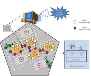
Fig. 1.2 A sample WSN diagram in an urban area

A sample wireless repeater network diagram is shown in Fig. 1.2, where wireless repeaters are deployed along city streets. An active communication

link has been established between two vehicles. All wireless repeaters on this

(24)

11

The technical challenges of routing protocol design in WSN remain in 3 aspects:

energy saving, multipath routing, and data-processing capabilities. Until now extensive efforts have been put into design of energy efficient routing solutions,

because sensor nodes can only have limited battery power. However, in the

future, if these nodes can utilize natural power (solar or wind energy), the design of routing protocols can foresee a big improvement. Also, because

sensor nodes lack of data processing and data storage units, they cannot

compute and memorize complex data structures. A common case is to store these routing information into a sink unit (or base station), which manages a

group of sensors adjacent to it. Distributed routing strategy is not suitable for

today’s WSNs, but they will be the future solution.

1.4 CONFERENCES AND ORGANIZATIONS

On 2nd of June 2013, the 5th International Symposium on Wireless Vehicular

Communications (WIVEC) was held in Dresden, Germany [1.30]. In its ‘calling for papers’ section, the following areas were shown great interest:

1. Antenna design, physical layer and propagation models

2. Radio resource management and interference management

3. Vehicular Networking Architectures

4. Networking protocols (including ad-hoc communication, routing,

geo-casting, etc.) and their evaluation

5. Simulation of Vehicular Communications Systems

6. QoS and cross-layer optimization design

7. Security, liability and privacy

(25)

12

9. In-car electronics and embedded integration of wireless vehicular

communications

10.Roadside infrastructure

11.Mobility management, mobility and vehicle traffic models

12.Digital maps and location technologies

13.Human Machine interface

14.Applications (eCall, eTolling, traffic information systems, safety

applications, wireless diagnosis, etc.)

15.Standards development, business models, policies

16.Assessment of impact on transport efficiency and safety

The Panel of this conference addressed the importance of VANET as below:

“VANETs—from research to initial deployment—what comes next? Vehicular ad hoc networks (VANETs) have been subject to research for

more than a decade now. Standardization development organizations in

Europe and North America have already released an initial set of VANET standards. Field operation tests are currently being carried out. Industry

consortia are now planning deployment of the first basic system. Based on

different viewpoints and experiences from recent research studies, field trials and ongoing standardization process, the panel will discuss the

remaining and next steps towards full deployment and aims to conclude on

the coming key research questions. The panel with prominent speakers

from academia as well as industry covers radio, communication protocols, applications and security.”

(26)

13

Vehicular Technology (TVT) is an important section in the IEEE

Transactions series, mainly targeting on the following areas:

1. Mobile communications

2. Transportation systems

3. Vehicular electronics

In 2010, this journal received 486,646 downloads in the IEEE Xplore usage,

ranking 21st among 288 IEEE journals. Its impact factor has been

increasing steadily since 2004, as shown in table 1.2.

Table 1.2. Impact Factor of TVT [1.31]

Year 2004 2005 2006 2007 2008 2009 2010

IF 0.611 0.860 1.071 1.191 1.308 1.488 1.490

Furthermore, IEEE defined a series of industrial standards on vehicular ad

hoc networks, such as:

 1609.3-2010 Wireless Access in Vehicular Environments (WAVE):

Networking Services

(27)

14

Over-the-Air Electronic Payment Data Exchange Protocol for Intelligent Transportation Systems (ITS)

As can be seen from the facts above, the research society of VANETs is still

active and productive. The major contributions it provides are not only academic, but also targeting on daily life. Extensive research interests have

been put into interactions between personal devices to landmarks

(vehicles, skyscrapers, etc). It also helps in standardization of VANETs.

1.5 CONCLUSIONS

This has firstly reviewed the emergence and development of wireless

networks. Then a brief introduction was given to a special wireless network: the VANET. Since 2000s, enormous research efforts have been

put on it because of its importance to urban life. In this research, the

primary study is of a type of VANET consisting of ad hoc networks and WSNs, so a literature review was given for both of them. Since routing

protocol design is the main concern here, the current status of routing

protocols in each type of network was examined. Finally, the major research bodies (international conferences and IEEE societies) have been

listed to keep track of newest information and research focus.

From this chapter it may be concluded that a novel and reliable VANET routing system requires consideration of the network characteristics. An

ad hoc network is too random to describe a VANET, while a WSN is too

rigid to track vehicle movement. A novel idea is to combine an ad hoc network with a WSN, and this type of hybrid network will be sufficient to

(28)

15

one single routing protocol which suits this hybrid network, so one has

been developed in this thesis from a prototype mentioned in section 2.4. This network model is then optimized by evolutionary programming

technique, which is extensively described in chapter 4. Also a second

network architecture, based on stochastic geometry technique has been presented, in Chapter 5. Finally in chapter 6 a third network simulation

model: small world architecture is presented to solve VANET routing

problem. Comparison between these techniques implies that EP’s performance exceeds the other techniques with detailed positioning

information of mobile nodes available. This requires mobile nodes to have

Global Positioning System (GPS) capability. Stochastic Geometry is more

advantageous in predicting data loss rates of a certain link within an urban area with a constant node density. It provides feedback of average signal

loss rate, which is beneficial for optimization algorithms. Small World

technique requests additional network equipment and it changes network topology as well. However it simplifies the network architecture by adding

long range communication links to the system. So it reduces the average

hop count needed to establish a random communication, and improves the signal quality of it. To summarize, EP provides a cost effective solution to

optimize signal quality of VANET, SG is an alternative statistic model to

predict data loss rate and SW can be considered when long range

communication equipment is in presence.

REFERENCES

1.1C. Makaya and S. Pierre, Emerging wireless networks: concepts, techniques,

(29)

16

1.2W. R. Young, AMPS Introduction, Background, and Objectives, Bell Systems

Technical Journal, vol. 58, 1, pp. 1-14, Jan. 1979.

1.3G. de la Roche, A. A. Glazunov, B. Allen, LTE-advanced and next generation

wireless networks: channel modeling and propogation. Book ISBN:

9781119976707. Wiley, 2013.

1.4C. Zhu and Y.N. Li, Advanced video communications over wireless

networks, Book ISBN: 9781439880005, CRC Press, 2013.

1.5D. B. Green, A. S. Obaidat, An accurate line of sight propagation performance model for ad-hoc 802.11 wireless LAN (WLAN) devices,

Communications, 2002. ICC 2002. IEEE Conf. Vol. 5. 2002.

1.6J. C. Liberti, T. S. Rappaport, A geometrically based model for line-of-sight

multipath radio channels. Vehicular Technology Conference, Mobile Technology for the Human Race, IEEE 46th_{vol. 2, 1996.}

1.7D.A. Magder, P. Bosch, T. Klein, P. Polakos, L. Samuel, H.Viswanathan,

911-NOW: a network on wheels for emergency response and recovery operations, Bell Labs Technical Journal, vol. 11, no. 4, pp 113-133, 2007.

1.8W. Enkelmann, FleetNet-applications for inter-vehicle communication,

Proceedings of the IEEE Intelligent Vehicles Symposium, pp. 162-167, 2003. 1.9D. Reichardt, M. Miglietta, L. Moretti, P. Morsink, W. Schulz, CarTALK2000:

safe and comfortable driving based upon inter-vehicle communication.

Intelligent Vehicles Symposium, 2002. Proceedings. IEEE, pp 545-550,

2002.

1.10 F. Li and W. Yu, Routing in vehicular ad hoc networks: A survey. IEEE

Vehicular Technology Magazine, vol. 2, no. 2, pp. 12-22, 2007.

1.11 Y. Toor, P. Muhlethaler, and A. Laouiti, Vehicle Ad Hoc networks: applications and related technical issues, IEEE Communications Surveys

(30)

17

1.12 J. Loo, J. L. Mauri and H. Ortiz, Mobile ad hoc networks: current status

and future trends, Book ISBN: 9781439856505, CRC Press, 2012.

1.13 F. F. Kuo, The ALOHA system, ACM Computer Communication Review:

vol. 25, 1995.

1.14 T. Cooklev, Wireless communication standards: a study of IEEE 802.11, 802.15 and 802.16. Book ISBN: 9781118098837. IEEE Press, 2004.

1.15 E. M. Royer, C.K. Toh, A review of current routing protocols for Ad Hoc

mobile Wireless Networks, pp 46-55, IEEE Personal Communications, April 1999.

1.16 C. E. Perkins and P. Bhagwat, Highly dynamic destination-sequenced

distance-vector routing (DSDV) for mobile computers, pp 234-244,

Computer Communications, October 1994.

1.17 C. C. Chiang, Routing in clustered multi-hop, mobile wireless networks

with fading channel, Proceedings of IEEE SICON, April 1997.

1.18 S. Murthy and J. J. Garcia-Luca-Aceves, ‘An Efficient Routing Protocol for Wireless Networks’, ACM Mobile Networks and App. J., Special Issue on

Routing in Mobile Communication Networks, pp. 183-97, 1996.

1.19 C. E. Perkins and E. M. Royer, ‘Ad-hoc On-Demand Distance Vector Routing,’ Proc. 2nd_{IEEE Workshop Mobile Comp. Sys. And Apps. , pp.}

90-100, 1999.

1.20 D. B. Johnson and D. A. Maltz, ‘Dynamic Source Routing Protocol for

Mobile Ad Hoc Networks,’ Mobile Computing, pp. 153-81, 1996.

1.21 V. D. Park and M. S. Corson, ‘A Highly Adaptive Distributed Routing

Algorithm for Mobile Wireless Networks,’ Proc. Infocom’97, Apr. 1997.

1.22 C-K. Toh, ‘A Novel Distributed Routing Protocol To Support Ad-Hoc Mobile Computing,’ Proc. 1996 IEEE 15th_{Annual Int’l. Conf., pp. 480-96,}

(31)

18

1.23 R. Dude et al., ‘Signal Stability based Adaptive Routing (SSA) for Ad-Hoc

Mobile Networks,’ IEEE Pers. Communications, pp. 36-45, 1997.

1.24 M. Gerla, C. –C. Chiang, and L. Zhang, ‘Tree Multicast Strategies in Mobile,

Multihop Wireless Networks,’, ACM/Baltzer Mobile Networks and Apps. J.,

1998.

1.25 J. N. Al-karaki, Ahmed E. Kamal, ‘Routing techniques in wireless sensor

networks: a survey,’ Wireless Communications, IEEE, Dec. 2004.

1.26 Y. Yu, D. Estrin, and R. Govindan, ‘Geographical and Energy-Aware Routing: A Recursive Data Dissemination Protocol for Wireless Sensor

Networks,’ UCLA Comp. Sci. Dept. tech. rep., UCLA-CSD TR-010023, May

2001.

1.27 I. Stojmenovic and X. Lin, ‘GEDIR: Loop-Free Location Based Routing in Wireless Networks,’ Int’l Conf. Parallel and Distrib. Comp. and Sys., Boston,

MA, Nov. 3-6, 1999.

1.28 F. Kuhn, R. Wattenhofer and A. Zollinger, ‘Worst-Case Optimal and Average-Case Efficient Geometric Ad Hoc Routing,’ Proc. 4th_{ACM Int’l. Conf.}

Mobile Comp. and Net., pp 267-78, 2003.

1.29 B. Chen et al., ‘SPAN: an Energy-efficient Coordination Algorithm for Topology Maintenance in Ad Hoc Wireless Networks,’ Wireless Networks,

vol. 8, no. 5, pp. 481-94, 2002.

1.30 5th_{International Symposium on Wireless Vehicular Communications,}

Dresden Germany, http://www.ieeevtc.org/wivec2013/index.php. Accessed 10th_{November 2013.}

1.31 IEEE Vehicular Technology Society, http://www.vtsociety.org/ .

(32)

19

1.32 Random Waypoint Model Matlab reference page:

(33)

20

CHAPTER 2 E V O L U T I O N A R Y P R O G R A M M I N G

In this chapter an overview of evolutionary programming (EP) is given, since

this is used as a major optimization tool in this research. EP assists the

algorithms designed evolve from a population of routing results to reach a near-optimum objective. EP has been proved in scientific research as a reliable

optimization tool. A literature review is firstly presented in section 2.1,

followed by the introduction of a series of recently developed EP variants. An emphasis will be placed on multiple objective optimization approaches in

section 2.2, which play a critical part in the research analysis. Finally, a specific

example in the area of Dense Wavelength Division Multiplexing (DWDM)

networking is reviewed in section 2.3 to illustrate EP in action.

2.1 HISTORY OF EVOLUTIONARY PROGRAMMING [2.1]

The term optimization comes from an idea to determine ‘a best’ solution to a certain mathematical problem. Such problems occur in many fields, such as

economics, management, physics and engineering. For example, in the

construction of buildings it is desirable to find an optimal solution to satisfy customer requirements with minimum material cost [2.2]. Furthermore, in

numerical analysis such as data fitting, the need to find an equation with an

optimal curve shape often arises. The solutions play a critical part in daily life,

and the process to discover these solutions is called optimization.

In recent times, the true beginning of the exploration of the solution of

(34)

21

series of equations of a variable x, with an order of n, from practical conditions.

Then, an optimization problem was transferred into a mathematical problem: to find either a local minimum or a local maximum value of x. However, this

method is not suitable to solve network routing optimization problems,

because a network (either for transportation or electrical current) may have hundreds or thousands of variables which results to an impossible number of

equations to solve. However, a method has it has been proposed [2.4] to use

evolutionary programming to solve network routing problems.

Evolutionary programming (EP) uses biology inspiration inherited from Darwin’s theory, which believes that species have the ability to evolve to fit

better in their environment in a gradual and natural way [2.5]. A critical

presumption of EP is that there exist multiple approaches to a given task, and yet these solutions all stand. The idea is to repeat a certain procedure on a

problem until a better or best solution termination condition is met. This is

necessary, especially on those puzzles which cannot be solved by conventional methods. EP will choose one of these approaches and match it with the

real-world environment.

EP is often referred to as a population-based optimization, because it generally consists of a population of many candidate solutions on a specific problem, and

as time passes, this population evolves to a better solution. Although very

similar to expert systems and being able to be classified as a member of the set of artificial intelligence methods [2.6], EP is different to classical expert

systems, or fuzzy logic sets, because these model deductive reasoning, while

evolutionary algorithms model inductive reasoning.

(35)

22

(bio-inspired intelligence). Ant colony optimization (ACO, [2.3]) is another

prominent algorithm, applied largely on Internet search engine design as well. However, some authors declare that they are not part of EP because they only

follow specific roles inherited from insect families.

2.2 MULTIPLE OBJECTIVE OPTIMIZATIONS

Recent advancements of EP include the following:

 Simulated Annealing [2.1]

 Ant Colony Optimization [2.3]

 Particle Swarm Optimization [2.2]

 Differential Evolution [2.1]

 Estimation of Distribution Algorithms [2.1]

 Biogeography-Based Optimization [2.6]

 Multi-Objective Optimization [2.7]

Multi-objective optimization is a hot topic in current scientific research. Many

real-world optimization problems are multi-objective, especially in

engineering design. For example, when wireless network architecture is designed, the engineer needs to consider how many access points need to be

placed to cover the whole area. The quantity of these access points is one

parameter to optimize, but the coverage of wireless signals is the other factor. Sometimes, the total energy saving of the network needs to be considered as

well. The problem of balancing signal coverage and material cost is a

multi-objective optimization problem.

(36)

23

A multiple objective optimization problem can be expressed as a function of x,

where x is n-dimensional:

( ) ( ) ( ) ( ) (2.1)

Multi-objective optimization process can be treated as a search of a Pareto optimal set, which consists of a set of Pareto optimal points:

⇔ { ( ) ( ) { ( )

( ) } (2.2)

The goal of a single-objective optimization algorithm is to find an optimal point which is a local minimum (or maximum) value of a certain fitness function.

However, in multiple objective optimizations, the goals of an algorithm might

be the following:

 Maximize the number of individuals that can be found within a

predefined Pareto set;

 Minimize the average distance between a candidate population set and

the objective Pareto set;

Sometimes the average distance, M, may be used to evaluate the fitness level of

a population. In section 2.3, a multiple objective optimization case is given.

2.3 EP IN DWDM NETWORK DESIGN

In this project, EP was applied as an optimization mechanism after an initial

path was given in a geographic map. The idea was to consider a known application of EP to optimize communication channels from previous work in

the area within the Warwick Intelligent Systems Engineering Laboratory [2.4].

(37)

24

 What is the performance of an EP-based optimization strategy when

the network receives multiple connection requests?

 How does the network behavior change when the Cost 239

configuration is replaced with an ad-hoc scenario (in simulation, a 40

node random network)?

The following sections first introduce this optimization process, and then

apply it to two different scenarios. After this, the performance of the strategy is

analyzed to ascertain its suitability for more dynamic and random network

environments.

2.3.1 Network Model

The benchmark network used in this paper is the Cost 239 Pan European Network (PAN) [2.4]: an optical fiber network connecting major European

cities. A diagram of which is shown in Fig 2.1 (Page 25). This network has 18

nodes and 69 links, with an average node degree of 3.83. The weight assigned

to each link is the actual physical distance between two cities in kilometers. It is assumed that before any algorithm initiates, no connections exist in the

network.

The creation of the dynamic connection is based on the scheduled traffic model previously utilized by Kuri et al. [2.5]. In this approach, the scheduled traffic

demands, CRi, are represented thus:

CRi = [s, d, c, Ts, Te], (2.3) where s and d are the source and destination node pair, c is the capacity

requested by this traffic (in terms of wavelengths), and Ts and Te are the

(38)

[image:38.595.126.501.73.497.2]

25

Fig. 2.1 European Cost239 Network—Topology with actual distances in km

Table 2.1 shows an example of a set of traffic requests expressed within this

scheduled traffic model.

Figure 2.2 illustrates three connection requests showing both their starting times and their tear down times. In addition, there is a capacity constraint on c

that arises both because there are clearly limited numbers of nodes and

wavelengths and because it is assumed here that the traffic is unidirectional. The latter reason results in half of the capacity of node s being reserved for

(39)

26

the allocation for traffic CRi on node s cannot exceed half of the maximum

capacities of all links originating from node s. Mathematically, for a number of links Ls connected to node s, each link supports up to K wavelengths [2.5],

(2.4)

The links in the COST 239 network are specified in Table 2.2, including, inter

alia, values for Ls.

In order to avoid blocking, the input process is assumed as follows:

For each node, before its capacity is full, the connection requests that originated

from it are treated with “immediate service”—no traffic congestion will be

caused from the starting point, but it is possible to get congestion at other nodes; A timer is set for the first connection request so that, once the node becomes

congested, this connection request will be dropped—the network links

allocated to it will be freed.

Table 2.1 Example of scheduled traffic requests

Connection

Requests

s D c Ts Te

CR0 15 5 6 1 3

CR1 17 3 1 2 4

CR2 3 8 3 3 6

CR3 17 6 4 4 9

A global resource lookup table is used to keep a record of every node’s available

links. This table is updated as soon as a new connection is assigned links and

wavelengths. Once the resource of a certain node is depleted, it will be marked

(40)

27 CR0

CR1

CR2

0 1 2 3 4 5 6 7 8 9 10 T

Fig. 2.2 Example of dynamic connection requests

(x-axis stands for time; y-axis stands for different requests)

An optimization process is executed after a certain period (e.g. 10 connections) to make global network resource allocation more efficient. This will also check

every node’s load capacity and make modifications to balance the load.

Table 2.2: Available links of each node in Cost 239 network

Node ID 1 2 3 4 5 6 7 8

Link No. 5 3 6 6 2 2 5 2

Capacity 20 12 24 20 8 8 20 8

Node ID 9 10 11 12 13 14 15 16

Link No. 5 3 2 2 3 4 7 3

Capacity 20 12 8 8 12 16 28 12

2.3.2 Path routing algorithm

In this section, a dedicated path protection scheme is applied to every existing

traffic connection to make sure they are protected in advance. A Dijkstra-shortest-path algorithm [2.6] is used to find a primary route and three backup

routes for each community. The backup path is designed with a backup path

(41)

28

Thus, full recovery is promised on primary paths for every existing connection

in this network.

Table 2.3: Example of Path Set Series

(s,d)pair 1, 17 2, 11 3, 10 5, 4 6, 10 8, 16

Path 1 1-9-17 2-9-15-11 3-15-10 5-16-18-4 6-15-10 8-17-7-16

Path 2

1-14-7-17

2-10-15-3-12-11

3-1-9-2-10

5-7-17-4

6-3-1-9-2-10

8-1-9-17-18-16

Path 3 1-8-17

2-13-4-15-11

3-7-17-4-13-10

5-9-4 6-13-10 8-5-16

Path 4

1-3-14-17

2-12-11

3-6-15-10

5-13-4 6-2-10 8-18-16

Table 2.3 gives examples of path sets and, as may be seen in the table, the search results from the Dijkstra algorithm successfully meet the survivability

requirement by providing three backup paths for each connection. However,

some backup paths are advantageous in capacity reduction, as well as link load

balance. Thus, it is possible to reduce total network capacity usage and balance link loads through the exchange of a primary path and its backup paths.

Fig. 2.3 Example of alternative path selection

Fig. 2.3 presents an example of multiple paths and the advantages of alternative

(42)

29

Dijkstra algorithm, whilst the dotted line paths represent backup paths. By

inspection, it is easily recognized that the path 5-9-4 has fewer hops compared with the primary path 5-16-18-4, and clearly fewer hops means reduced

capacity occupation. Backup path 5-9-4 is a better choice, for traffic where

capacity is the primary driver rather than pure transmission speed. Backup path 5-14 has the same hop length as the primary path but does share the link

7-17 with other traffic increasing the probability of blocking. In summary, backup

path 5-9-4 will be chosen for total network capacity optimization, and backup path 5-7-17-4 will not be chosen because of the increased risk of traffic blocking.

2.3.3 Genetic algorithm (GA)

A genetic algorithm (GA) [2.7] is a searching technique to find solutions of

optimization problems. It is a class of evolutionary algorithm which uses

techniques inspired by evolutionary biology such as inheritance, mutation and crossover. A general process flow chart of a GA is shown in Fig. 2.4, where the

GA simulates a problem solving process as a biological evolutionary path by involving population creation, population reproduction, and an offspring

selection process. For the path optimization issue, the path set found by the path

searching algorithm will be used as an initial population. The GA will cross over

(43)

[image:43.595.161.468.69.323.2]

30

Fig. 2.4 Flow chart of genetic algorithm process

To employ a GA, it is necessary to map the problem to a set of chromosomes that

represent the candidate solutions. In this application, the chromosomes (or

population) are encoded, as shown in Table 2.4:

Table 2.4 Example of chromosome encoding

The chromosome consists of 2n digits, where n is the number of live connections in a specific timeslot. In other words, 2 digits represent an existing connection in

network. The coding scheme represents different path orders, using 00 as the

primary path and 01, 10 and 11 as backup paths 1, 2 and 3.

2.3.4 Fitness function

To determine which solutions are the best, it is necessary to define a fitness

[image:43.595.132.503.465.543.2]

(44)

31

optimization, the fitness function is an objective function which calculates a

specific outcome (fitness value) from chromosomes. The value that is produced by the fitness function is used as the basis of the decision on whether or not a

given chromosome will survive into or produce offspring for the next

evolutionary generation. Later, this choice of progression to the next generation will be discussed, but first the optimization strategies employed in this work

will be described, along with their specific fitness functions.

A. Least-Loaded Routing (LLR)

This policy defines the fitness function as the total network capacity usage

under the traffic pattern contained in the chromosomes. The fitness value of a

certain chromosome represents the network wavelength resources allocated to the traffic connections, and the objective is to find a chromosome with the least

network usage. The target of this optimization approach is to minimize total

network resource capability allocated within all path candidates. The fitness function for capacity and length is:

∑ ∑ (2.5)

K is the number of existing connections in the network, and m is the number of

links contained in the ith_{chromosome. This function sums the total capacities}

used on individual links contained in a specified route, and assigns this value to

the route (chromosome) as an optimization target. To encompass all routes, the mean of all fitness values from a whole population is used and here this is

referred to as the AWUT (Average Wavelength Usage per Traffic), and is defined

below. The AWUT forms the target used to evaluate the ultimate optimal results

from traffic patterns in the simulations presented later.

(45)

32

This policy defines the fitness function as the network blocking probability

under the traffic pattern contained in the chromosomes. Here, the fitness value of a certain chromosome represents the probability that the traffic will

experience congestion on the current routes, and the objective is to find a

chromosome with the least congested route. In this optimization approach, the probability is minimized within all path candidates producing a fitness function:

∑ ∑ (2.6)

pi,j is the probability of congestion of the ith traffic flow congestion on the jth link,

calculated as:

(2.7)

where ci,j is the capacity allocated to the ith traffic flow on the jth link, and cmax is

the predefined maximum available capacity for the network. This means that as

one would expect, the more capacity that is used on a link, the higher the

probability will be that it will cause traffic congestion. This fitness function sums

the traffic congestion probabilities on individual links contained in a specified route, and assigns this value to the route (chromosome) as an optimization goal.

In this case, a target value termed the ANBP (Average Network Blocking

Probability) is applied in the simulations below to evaluate the ultimate optimal results from this pattern. The ANBP is the mean value of all LCR fitness values

from a whole population, and again its observation permits the monitoring of

the evolutionary process.

2.3.5 Crossover and mutation [2.7]:

(46)

33

new path sets for the same traffic. The appropriate fitness function is used to

evaluate whether the new path sets will be selected for the next generation.

Fig. 2.5: Crossover operation

An example of crossover operation is shown in Fig. 2.5, where paths are

allocated to two connection requests (1-17 and 2-11) using the path routing

algorithm. After encoding, chromosome parent 1 has the route set 1-14-7-17 for

traffic 1-17 and route set 2-9-15-11 for traffic 2-11, while chromosome parent 3 has the route set 1-8-17 for traffic 1-17 and route set 2-12-11 for traffic 2-11.

The crossover operation exchanges their second route set and generates

offspring 1 and 3. Offspring 1 is fitter than parent 1, since the total wavelength usage is reduced by 1 hop, so it will be selected for the next generation in LLR

policy. Also it decreases the congestion of link 2-9, 9-15 and link 15-11, but with

an addition of link 2-12 and 12-11, so it is necessary to calculate the global network congestion probability to see if it is better than parent 1 in the LCR

policy.

Mutation is the other genetic operator used to maintain genetic diversity from

one generation to the next by creating mutated chromosomes. In the simulation algorithm, it is designed as a triggered operation when an evolutionary process

(47)

34

operation selects the first constant bit, i.e. the position in which all

chromosomes have the same value and reverses it.

Fig. 2.6 Mutation operation

Figure 2.6 illustrates the generation of a mutated offspring that arises and

delivers a shorter route from node 1 to node 8. This operation is beneficial to the solution pool after a series of crossover operations, since it creates a

completely novel chromosome that contributes to the diversity of the

population.

2.4 SIMULATION RESULTS

Simulation setup

In order to fully address the algorithm’s efficiency, the simulation results are

presented in two parts. In part one, the performance of the algorithm under a

benchmark network scenario is analyzed. In part two, the algorithm is compared with two other conventional routing assignment techniques under

different network environments and with different traffic loads to illustrate

better a genetic algorithm’s advantages and disadvantages. All simulations were run on Windows XP with a 3.31 GHz CPU and the software platform was

MATLAB (version: 7.8.0.347, R2009a).

Part one: single network performance

Ten iterations of randomly-generated traffic requests were chosen as an initial

(48)

[image:48.595.143.460.142.669.2]

35

(49)

36

Each of the iterations contained ten connection requests with exactly the same

format as that shown in Table 2.1. The optimization results and observations concerning them are presented below, along with the ALR (Actual output versus

Limit Ratio) data record.

Average Wavelength Usage per Traffic (AWUT) optimization

As discussed before, the objective of the optimization algorithm within the LLR policy is to minimize the global network resource usage, and AWUT is a

performance criterion to reflect the algorithm efficiency. AWUT is defined as the

following:

∑ (2.8)

where N is the number of traffic streams existing in the network, Ci is the

capacity of ith_{stream, and L}_i_{is the link number of the primary route assigned to}

the ith_{traffic stream. The AWUT represents the average network resources}

(lightpaths/wavelengths) allocated per traffic stream in the primary path

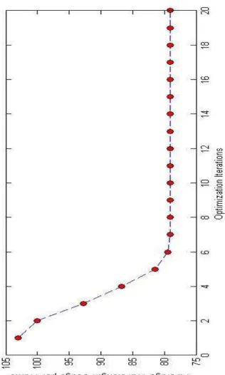
assignment. From Fig.2.7 (page 36) it is clearly shown that, after 6 iterations, the AWUT has decreased by 23.3% (from 103 to 79) and then has become stable. In

this case, the lower limit is 79, and the algorithm successfully reaches its

optimal outcome. An advantage of this optimization process is that it only needs

traffic information as input, and calculates the optimal paths according to local information. Compared with adaptive routing algorithms which need support

from the network signaling layer and an appropriate protocol in advance, the GA

simulates an environment in which best paths naturally evolve from a group of candidates, which can be calculated and stored by routers in advance.

(50)

37

ALR is a performance criterion for the optimization achievement, and it is

defined as the following:

(2.9)

where ALRi is the ALR value for ith iteration of optimization. Initiali is the ith

initial total network load, Actuali is the ith optimization result achieved by the

algorithm, and Mini is the ith lower limit of the algorithm known in advance.

Apart from several optimal cases, ALR (as shown in Fig. 2.8) is a constant value ranging from 70% to 90% for most of the optimization rounds. To achieve this

value the algorithm usually takes 8 to 12 iterations to optimize the path.

Compared with the simulation results in [19], the static optimization case, the

dynamic algorithm’s single-iteration performance (Fig. 2.7) is superior (23.3% versus 7.1%), but the average performance over a long time is similar. The

optimization performance of the GA relies heavily on the nature of the path

set—its population, and the higher the deviation the path sets have, the better the optimization result the GA can achieve.

(51)

38

However, the advantage of the GA is apparent in that the number of iterations

needed to reach the optimal value, given a certain network topology, is almost constant, no matter what the nature of the traffic is, and what complexity its

route involves for calculation. The optimization speed depends on the crossover

population size versus the total population size. In the simulation environment, the crossover population size is 20, and the total population size is 4K, where K

is a variable, represents existing connection numbers. In case of Fig. 2.7, where

K = 7, the population size is 16384, then the GA optimization has the same effect

with 2730 ordinary ranking and sorting operations, and a single crossover

operation has the same effect with 273 such operations. From this point of view,

implementing GA will greatly accelerate the speed of path routing in DWDM

network.

Traffic Blocking Probability (TBP) optimization

TBP is another optimization objective within the LCR policy, and its mathematical expression is as follows:

( ) (2.10)

where BPi is ith route blocking probability:

(2.11) where cl is allocated capacity (in wavelength) of the lth link in ith route, and cmax is

the maximum capacity of each link. The traffic blocking probability is the

maximum value among its individual traffic blocking probabilities which are presented by peak values from their link blocking probabilities.

The calculation of the TBP makes use of a global resource lookup table

(mentioned in dynamic connection creation, section II: Methodology), which

(52)

39

where s and d represent the source and destination pairs for link Li, and Ci is the

allocated link capacity. Fig. 2.9 gives an example of a TBP optimization result:

Fig. 2.9 TBP optimization result after 8 iterations

It is worth noting that the value of the TBP not only serves as a warning for individual links when they reach maximum capacity, but also represents a

capacity occupation level for the entire network, given the in situ capacity

allocation condition for all links. If the value of the TBP is below 0.5, the network should to be in good condition, with more than half link capacities being free for

future traffic. An effective operation in TBP reduction (as shown in Fig. 2.9) is to

reallocate traffic from more congested paths to less occupied paths, thus achieving an overall optimal result. From Fig. 2.9 it may be seen that the

simulation successfully decreased overall TBP from 1 to 0.1 after 7 iterations.

Part two: comparative results

In order to fully evaluate the performance of the GA under different network

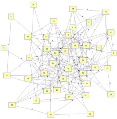
scenarios, a 40 node Gaussian distributed network was created (shown at Fig.

2.10) as a counterpart to the Cost 239 network. Two commonly-used searching techniques were used as benchmarks:

(53)

40

[image:53.595.139.501.122.466.2]

 Directly Relative Capacity Loss (DCRL)[2.9]

Fig. 2.10 Gaussian distributed 40-node network

The FF strategy simplifies the wavelength assignment procedure into a “first come first serve” process: the first incoming traffic is assigned the first available

wavelength within the wavelength index, and when no more wavelengths are

available, the traffic is blocked. In the DRCL strategy, each node stores information on the capacity loss on each wavelength in its own lookup table.

This table is called the Relative Capacity Loss table and whose content is a triple

of wavelength, destination, and RCL weight. When a connection request arrives and more than one wavelength is available on the light path, DRCL will make use

of the RCL table and calculate the path which has a minimum RCL weight among

(54)

41

Table 2.5 comparison of FF, DRCL and GA using four wavelengths and