An Efficient Algorithm for the Numerical Computation of the Complex Eigenpair of a Matrix

(1)

http://www.scirp.org/journal/jamp ISSN Online: 2327-4379

ISSN Print: 2327-4352

An Efficient Algorithm for the Numerical

Computation of the Complex

Eigenpair of a Matrix

R. O. Akinola

*

, K. Musa, I. A. Nyam, S. Y. Kutchin, K. V. Joshua

Department of Mathematics, Faculty of Natural Sciences, University of Jos, Jos, Nigeria

Abstract

In computing the desired complex eigenpair of a matrix, we show that by adding Ruhe’s normalization to the matrix pencil, we obtain a square nonli-near system of equations. In this work, we show that the corresponding Jaco-bian is non-singular at the root and that with an appropriately chosen initial guesses, Ruhe’s normalization with a fixed complex vector not only converges quadratically but also faster than the earlier Algorithms for the numerical computation of the complex eigenpair of a matrix. The mathematical tools used in this work are Newton and Gauss-Newton’s methods.

Keywords

Quadratic Convergence, Newton’s Method

1. Introduction

In [1], Akinola and Spence considered the problem of computing the eigenpair

(

x,λ

)

from the generalized complex eigenvalue problem:

,

λ

=

Dx

Px

(1)

where ∈ n, ≠0,λ∈ ,

x  x  D is a large real n n× non-symmetric matrix and

P a real symmetric positive definite matrix. After adding the normalization [2]

1,

H ₌

x Px

(2)

to (1), they obtained a combined system of equations of the form F

( )

u =0,

where  H,

λ

,

=  

u x given as

( )

(

₁

)

₁ 0.

2 2

H

F

x

λ

 − 

 

=_ _=

− +

 

 

D P x

u

Px

(3)

How to cite this paper: Akinola, R.O., Musa, K., Nyam, I.A., Kutchin, S.Y. and Joshua, K.V. (2017) An Efficient Algorithm for the Numerical Computation of the Com-

plex Eigenpair of a Matrix. Journal of

Ap-plied Mathematics and Physics, 5, 680-692.

https://doi.org/10.4236/jamp.2017.53057

Received: December 28, 2016 Accepted: March 21, 2017 Published: March 24, 2017

http://creativecommons.org/licenses/by/4.0/

(2)

In trying to solve the nonlinear system (3), two drawbacks were encountered. The first one is that if x from

(

x,λ

)

solves (3), then so does expiθx for any

[

0, 2π

)

θ ∈ , which means that x has no unique solution. Secondly,

x

in

T

H ₌

x x is not differentiable since

x

does not satisfy the Cauchy-Riemann [3] equations which implies that (3) cannot be differentiated and the standard Newton’s method cannot be applied. The author then proposed that the above drawbacks could be overcome at least for the P=I case. Before the works of

Akinola, Ruhe [4] and Tisseur [5] added the differentiable normalizations

1,

H ₌

c x (4) and

T

, s

τe x=τ

(5)

where c is a fixed complex vector and

τ

=max

(

D , P

)

for some fixed s. Adding each of the two normalization to (1), Ruhe and Tisseur then obtained the following combined system of equations;

( ) (

)

0,

1 H

F =_ −λ _=

−

 

D P x u

c x (6)

and

( ) (

T

)

0,

s

F λ

τ τ

 − 

=_ _=

−

 

D P x u

e x (7)

which have the corresponding Jacobians

( ) (

)

,

0

u H

F =  −λ − _

 

D P Px u

c (8)

and

( ) (

T

)

.

0 u

s

F λ

τ

 − − 

=  

 

D P Px u

e

(9)

In this paper, we show that the square Jacobian given by (8) is nonsingular at the root using the ABCD lemma if the eigenvalue of interest is algebraically sim-ple. The major distinction between the two-norm normalization and Ruhe’s normalization is that the two-norm normalization is a natural normalization which makes the choice of c free. The Jacobian (9) above was shown to be singular in [5] at the root if and only if λ∗_{is a finite multiple eigenvalue of the}

pencil

(

D P,

)

.

(3)

The plan of this paper is as follows: in Section 2, we used Keller’s ABCD Lemma [8] to show that the Jacobian (8) is nonsingular at the root in Theorem 2.1 and we present the four Algorithms. In Section 3, we compare the performance of the four algorithms on three numerical examples. Eigenvalues are used in diffe-rential equations in studying stability and in complex biological systems in de-termining eigenvector centrality (see also [9] [10]).

2. Methodology

In this section, we proof the main result in this paper which states the condition under which the Jacobian matrix (8) (for P=I) is non-singular at the root, that is x∗ =

(

x∗,

λ

∗

)

. This is then followed by a presentation of Algorithm 1,

which is actually Newton’s method for solving (6). The remaining algorithms have been discussed extensively in [1] [6] and [7]. For the sake of avoiding self plagiarism, we refer the interested reader to those articles.

Algorithm 1 involves solving an

(

n+1

)

by

(

n+1

)

square system of

equa-tions using LU factorisation and does not involve splitting the eigenvalue and eigenvector into real and imaginary parts.

Algorithm 2 involves splitting the eigenpair into real and imaginary parts to obtain an under-determined non linear system of equations. This results in solving a

(

2n+1

)

real under-determined linear system of equations for

(

2n+2

)

real

unknowns using Gauss-Newton method [11]. This is solved using QR factorisation. Algorithm 3 also involves splitting the eigenpair into real and imaginary parts but with the help of an added equation we obtained a square

(

2n+2

)

by

(

2n+2

)

system of linear equations which is solved using LU factorisation.

Algorithm 4 is closely related to Algorithm 1 in the sense that both uses complex arithmetic. While Algorithm 1 used a fixed complex vector which does not change throughout the computation, Algorithm 4 uses the natural two-norm normalization which ensures that the eigenvector is updated at each stage of the computation.

Theorem 2.1. Let

(

₋

λ

∗

)

D I be an n by n matrix, , n

C

∗ _∈

x c . Let

(

)

_,

0 H

λ∗ ∗

 − − 

=  

 

 

D I x

M

c

(10)

be an

(

n+1

)

by

(

n+1

)

matrix. If D−λ∗I is singular and rank

(

D−

λ

∗I

)

=

1 n

−

, then M is nonsingular if and only if ψH_x∗_≠0, for all

(

λ∗

)

H \ 0

{ }

∈ −

ψ  D I and cHφ≠0, for all

φ

∈

(

D−

λ

∗I

)

\ 0

{ }

. Where

(

₋

λ

∗

)

D I

 is the nullspace of ₋λ∗

D I.

Proof: Let M be nonsingular. Assume D−λ∗I is singular and cHφ=0,

we want to show by contradiction that _cHφ_≠0. We multiply _M from the

right by the nonzero vector

[ ]

φ

, 0H to yield

(

)

(

)

0

.

0 0

0

H H

λ φ λ φ

φ

∗ ∗ ∗

 − −    −   

= =

 _{ }   _{ }

      

   

D I x D I

c c (11)

(4)

contradic-tion, hence _cHφ_≠0. Similarly, let ψ xH ∗ ₌₀, multiply _M from the left by

the nonzero vector

[ ]

ψ

, 0H to obtain

[

0

]

(

)

(

)

0 0 .

0

H H H H

H

λ

ψ _ − ∗ − ∗_₌_ ₋λ∗ ₋ ∗_₌_ _

 

 

 

D I x

ψ x

ψ D I

c

This shows that M is singular, contradicting the nonsingularity of M, therefore, ψ xH ∗ _≠0.

Conversely, let ₋λ∗

D I be singular of rank

(

D−

λ

∗I

)

= −n 1, and assume

0 H ∗ _≠

ψ x and _cHφ_≠0. We want to show that _M is nonsingular. If we can

show that the vector

[ ]

p,q H is zero in

(

)

_,

0 0

H _q

λ∗ ∗

 − −    

=

 _{    }

     

 

D I x p

c

0

then M is nonsingular. After expanding the above equation, we obtain

(

D−

λ

∗I p

)

−qx∗=0 (12)

0.

H ₌

c p (13) By using the fact that ψ DH

(

−

λ

∗

)

=0H

I in H

(

)

(

H

)

0

q

λ

∗ ∗

− − =

ψ D I p ψ x , we have q

(

ψ xH ∗

)

=0. But by assumption, ψ xH ∗ _≠0, hence _q=₀. With this

value of

q

, we are left with

(

D−

λ

∗I p

)

=0 in (12) and because D−λ∗I is singular, this implies that p=αφ. After substituting the value of

p

into (13), we have α φcH =0 from which

α =

0

is immediate since cHφ≠0.

There-fore, p=0 and M is nonsingular.

Next, we present Algorithm 1 for computing the complex eigenpair of D using complex arithmetic. This is the main contribution to knowledge in this paper.

Algorithm 1 Eigenpair Computation using Newton’s method

Input: ( )0 ( )0 T max , =  ,λ _ ,k

D x c and tol.

1: for k=0,1, 2,, until convergence do 2: Compute the LU factorisation of

( )

(

)

( ) . 0 k k H λ  − −       

D I x

c

3: Form

( )

(

( )

)

( ) ( ) . 1 k k k k H λ  −  = −    −   

D I x

d

c x

4: Solve the lower triangular system ( )k ( )k Ly =d for ( )k

y .

5: Solve the upper triangular system ( )k ( )k

U∆v =y for ∆v( )k. 6: Update ( )k+1₌ ( )k _{+ ∆} ( )k

x x x .

7: end for Out for: (kmax)

v .

Stop Algorithm 1 as soon as ∆v( )k ≤tol.

(5)

Algorithm 2 Eigenpair Computation using Gauss-Newton’s method [1]

Input: D, ( ) ( ) ( ) ( ) ( )

T

0 0 0 0 0

1 , 2 ,α β, ,kmax

 

=  

v x x and tol.

1: for k=0,1, 2,, until convergence do

2: Find the reduced QR factorisation of

( )

( )k T= v

F v QR.

3: Solve T ( )k _{= −}

( )

( )k

R g F v for ( )k

g .

4: Compute _∆ ( )k ₌ ( )k

v Qg for ∆v( )k.

5: Update ( )1 ( ) ( )

.

k+ ₌ k _{+ ∆} k

v v v

v .

Algorithm 3 Eigenpair Computation using Newton’s method [6]

Input: ( )0 ( )0 ( )0 ( )0 ( )0 ( )0 ( )0 T

1 2 max

, =_ , _, =_ ,α β, _ ,k

D w x x v w and tol.

1: for k=0,1, 2,_{until convergence do}

2: Compute the LU factorisation of

( )

T

0 0 .

0 0  ₋    −        

M w Jw

w

Jw

3: Form

( ) 1

(

T

)

1 . 2 0 k −       = −       Mw

d w w

4: Solve the lower triangular system Lc( )k =d( )k for ( )k c .

5: Solve the upper triangular system U∆v( )k =c( )k for _∆ ( )k v .

6: Update ( )k+1 ₌ ( )k _{+ ∆} ( )k.

v v v

7: end for

Out for: (max) (max) (max) (max) T

, ,

k  k αk βk 

=  

v w .

Algorithm 4 Eigenpair Computation using Newton’s method in complex arithmetic [7]

Input: ( ) ( ) ( )

T

0 0 0

1 max

, =  ,λ _ ,k

D v x and tol.

1: for k=0,1, 2,, until convergence do

2: Compute the LU factorisation of

( ) ( ) ( )

( )

. 0 k k H k λ  − −    −   

D I x

x

3: Form ( )

( )

(

)

( ) ( ) ( ) . 1 1 2 2 k k k

kH k

λ  −    = − ₋ ₊     

D I x d

x x

4: Solve the lower triangular system ( )k ( )k Ly =d for ( )k

y .

5: Solve the upper triangular system ( )k ( )k

U∆v =y for ∆v( )k. 6: Update ( )k+1 ₌ ( )k _{+ ∆} ( )k.

v v v

v .

3. Numerical Experiments

(6)

2, Algorithm 3 and Algorithm 4) which were presented in the last section on three numerical examples. Throughout this section ( ) 1( ) , 2( )

k  kT kT

=  

w x x and

( ) ( ) ( )

,

k _α k _β k 

=  

λ .

Example 3.1. Consider the matrix

0 1

. 1 0 D=  _

−

 

We compared the performance of the four algorithms on the two by two matrix and the results are as presented in Table 1, Table 2, Table 3 and Table 4 respec-tively. In all four algorithms we used the same initial guesses ( )0 3

6.0 10

α ₌ _× − _,

( )0 1

9.9 10 i

β

₌ _× − _, ( )0 1 1

,

0 0 i

    =_{   }+    

[image:6.595.208.540.294.380.2]

x and c=

(

A+iI

)

. It was observed that

Table 1. Values of ( )k ( )k

i

α + β for the two by two matrix using Algorithm 1.

k ( )k ( )k

i

α +β ( )k+1₋ ( )k

x x _λ( )k+1₋_λ( )k _∆ ( )k

v

( )

( )k

F v

0 6.00000e−03+9.90000e−01i 1.7e+02 2.0e+00 1.7e+02 2.7e+00

1 1.41739e+00+2.39290e+00i 1.7e+02 3.7e+00 1.7e+02 3.4e+02

2 7.08322e−14−1.00000e+00i 3.2e+02 1.4e−13 3.2e+02 6.3e+02

[image:6.595.208.541.427.560.2]

3 4.90140e−16−1.00000e+00i 2.2e−11 5.4e−16 2.2e−11 4.4e−11

i

α + β for the two by two matrix using Algorithm 2. Quadratic convergence is shown in columns 4, 6 and 7 for k=3,k=4 and k=5.

k α( )k _β( )k (k+1)₋ ( )k

w w _λ( )k+1 ₋_λ( )k _∆ ( )k

v

( )

( )k

F v

0 6.00000e−03 0.99000 1.1e+00 1.8e−02 1.1e+00 2.1e+00

1 3.09120e−03 1.00505 4.2e−01 4.3e−03 4.2e−01 6.4e−01

2 8.65482e−04 1.00141 8.2e−02 1.5e−03 8.2e−02 8.9e−02

3 6.54625e−05 1.00011 3.4e−03 1.2e−04 3.4e−03 3.4e−03

4 2.19153e−07 1.00000 5.6e−06 4.2e−07 5.7e−06 5.7e−06

5 1.23636e−12 1.00000 1.6e−11 2.4e−12 1.6e−11 1.6e−11

[image:6.595.210.540.608.739.2]

6 4.04413e−18 1.00000 7.9e−17 1.0e−18 7.9e−17 1.6e−16

Table 3. Values of _α( )k _and β( )k _{for the two by two matrix using Algorithm 3.} Qua-dratic convergence is shown in columns 4, 6 and 7 for k=3, 4 and k=5.

k α( )k β( )k (k+1)₋ ( )k

w w _λ( )k+1 ₋_λ( )k _∆ ( )k

v

( )

( )k

F v

0 6.00000e−03 0.99000 1.1e+00 1.8e−02 1.1e+00 2.1e+00

1 3.09120e−03 1.00505 4.2e−01 4.3e−03 4.2e−01 6.4e−01

2 8.65482e−04 1.00141 8.2e−02 1.5e−03 8.2e−02 8.9e−02

3 6.54625e−05 1.00011 3.4e−03 1.2e−04 3.4e−03 3.4e−03

4 2.19153e−07 1.00000 5.6e−06 4.2e−07 5.7e−06 5.7e−06

5 1.23636e−12 1.00000 1.6e−11 2.4e−12 1.6e−11 1.6e−11

(7)

[image:7.595.55.543.94.663.2]

i

α + β for the two by two matrix using Algorithm 4. Quadratic convergence is shown in columns 3, 5 and 6 for k=3, 4 and k=5.

k ( )k ( )k

i

α + β ( )k+1₋ ( )k

x x _λ( )k+1₋_λ( )k _∆ ( )k

v

( )

( )k

F v

0 6.00000e−03+9.90000e−01i 1.1e+00 1.8e−02 1.1e+00 2.1e+00

1 −3.09120e−03+1.00505e+00i 4.2e−01 4.3e−03 4.2e−01 6.4e−01

2 −8.65482e−04+1.00141e+00i 8.2e−02 1.5e−03 8.2e−02 8.9e−02

3 −6.54625e−05+1.00011e+00i 3.4e−03 1.2e−04 3.4e−03 3.4e−03

4 −2.19153e−07+1.00000e+00i 5.6e−06 4.2e−07 5.7e−06 5.7e−06

5 −1.23633e−12+1.00000e+00i 1.6e−11 2.4e−12 1.6e−11 1.6e−11

6 1.68283e−17+1.00000e+00i 0.0e+00 8.4e−18 7.6e−17 1.5e−16

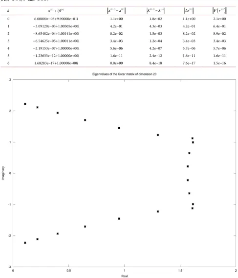
Figure 1. Distribution of the complex eigenvalues of the 20 by 20 grcar matrix. The x-axis is the real axis while the y-axis is the

imaginary axis.

(8)

Example 3.2.

The grcar matrix [12] [13] is a non symmetric matrix with sensitive eigenva-lues and defined by

( )

1, if 1

, 1, if and

0, Otherwise.

i j

i j i j j i k

− = +

 

= ≤ ≤ +

  D

Figure 1 shows the distribution of the complex eigenvalues of the twenty by twenty grcar matrix on the real and imaginary axis. All the four algorithms discussed in the last section converged to the eigenvalue 1

1.58207 6.43690 10 i

λ∗₌ ₊ _× − _after

[image:8.595.62.539.248.699.2]

12 iterations with the same starting guesses as shown in Table 5, Table 6, Table 7 and Table 8. However, unlike the first example in which Algorithm 1 con-verged faster than the other three, that was not the case, maybe due to the sensi-tivity of its eigenvalues.

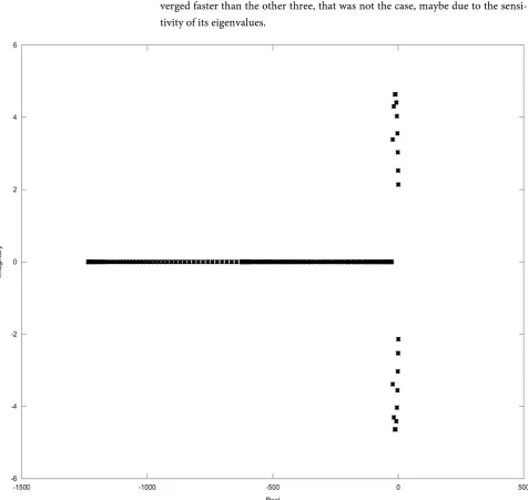
Figure 2. Distribution of the complex eigenvalues of the 200 by 200 bmw 200.mtx matrix. The x-axis is the real axis while the y-

(9)

Example 3.3.

Consider the 200 by 200 matrix D bwm200.mtx from the matrix market li-brary [14]. It is the discretised Jacobian of the Brusselator wave model for a chemical reaction. The resulting eigenvalue problem with P=I was also stu-died in [9] and we are interested in finding the rightmost eigenvalue of D which is closest to the imaginary axis and its corresponding eigenvector. Figure 2 shows the distribution of the complex eigenvalues of the matrix.

For this example, in all four algorithms we take ( )0 ( )0

0.0, 2.5

α

=

β

= in line

with [9] and took ( )0

1 =1 2 1

x , ₂( )0 31 1 2

=

x and 1 1

2 1i

= +

[image:9.595.211.539.272.482.2]

c , where 1 is

i

α + β for the twenty by twenty grcar matrix using Algorithm 1. Quadratic convergence is shown in columns 3 and 5 for k=10 and 11.

k ( )k ( )k

i

α +β ( )k+1₋ ( )k

x x _λ( )k+1₋_λ( )k _∆ ( )k

v

( )

( )k

F v

0 9.00000e−02+2.00000e−01i 1.2e+00 1.3e+00 1.8e+00 2.2e+00

1 1.08132e+00+1.08186e+00i 1.5e+00 2.6e+00 3.0e+00 1.6e+00

2 3.72785e+00+9.63132e−01i 9.1e−01 1.3e+00 1.6e+00 4.0e+00

3 2.47494e+00+7.62445e−01i 5.7e−01 7.6e−01 9.4e−01 1.2e+00

4 1.71950e+00+7.19775e−01i 7.6e−01 4.6e−01 8.9e−01 4.3e−01

5 1.26075e+00+7.25835e−01i 3.7e−01 3.1e−01 4.8e−01 3.5e−01

6 1.56634e+00+7.38078e−01i 3.1e−01 1.6e−01 3.5e−01 1.1e−01

7 1.62480e+00+5.86198e−01i 1.1e−01 6.7e−02 1.3e−01 5.1e−02

8 1.58877e+00+6.42286e−01i 1.9e−02 6.8e−03 2.0e−02 7.7e−03

9 1.58214e+00+6.43859e−01i 4.3e−04 1.8e−04 4.6e−04 1.3e−04

10 1.58207e+00+6.43690e−01i 2.1e−07 7.1e−08 2.2e−07 7.8e−08

[image:9.595.208.539.528.732.2]

11 1.58207e+00+6.43690e−01i 4.6e−14 1.9e−14 4.9e−14 1.5e−14

i

α + β for the twenty by twenty grcar matrix using Algorithm 2. Quadratic convergence is shown in columns 4, 5 and 6 for k=9,10 and 11.

k α( )k β( )k (k+1)₋ ( )k

w w _λ( )k+1₋_λ( )k ∆ ( )k

v

( )

( )k

F v

0 9.00000e−02 0.20000 7.6e−01 1.4e+00 1.6e+00 2.0e+00

1 1.49489e+00 0.11791 1.1e+00 1.1e+00 1.5e+00 1.1e+00

2 2.03853e+00 1.09037 5.5e−01 5.1e−01 7.5e−01 1.3e+00

3 1.70500e+00 0.69852 4.6e−01 3.2e−01 5.6e−01 3.2e−01

4 1.50162e+00 0.45319 5.5e−01 3.8e−01 6.7e−01 1.8e−01

5 1.84080e+00 0.63082 3.1e−01 1.9e−01 3.6e−01 2.6e−01

6 1.66945e+00 0.55208 1.5e−01 1.3e−01 2.0e−01 7.6e−02

7 1.55071e+00 0.60360 7.0e−02 5.4e−02 8.9e−02 2.3e−02

8 1.58816e+00 0.64225 7.9e−03 6.2e−03 1.0e−02 4.5e−03

9 1.58207e+00 0.64358 1.4e−04 1.1e−04 1.8e−04 5.9e−05

10 1.58207e+00 0.64369 3.0e−08 2.1e−08 3.7e−08 1.8e−08

(10)

[image:10.595.208.540.105.313.2]

i

k _α( )k β( )k (k+1)₋ ( )k

w w ( )k+1 ₋ ( )k

λ λ _∆ ( )k

v

( )

( )k

F v

0 9.00000e−02 0.20000 7.6e−01 1.4e+00 1.6e+00 2.0e+00

1 1.49489e+00 0.11791 1.1e+00 1.1e+00 1.5e+00 1.1e+00

2 2.03853e+00 1.09037 5.5e−01 5.1e−01 7.5e−01 1.3e+00

3 1.70500e+00 0.69852 4.6e−01 3.2e−01 5.6e−01 3.2e−01

4 1.50162e+00 0.45319 5.5e−01 3.8e−01 6.7e−01 1.8e−01

5 1.84080e+00 0.63082 3.1e−01 1.9e−01 3.6e−01 2.6e−01

6 1.66945e+00 0.55208 1.5e−01 1.3e−01 2.0e−01 7.6e−02

7 1.55071e+00 0.60360 7.0e−02 5.4e−02 8.9e−02 2.3e−02

8 1.58816e+00 0.64225 7.9e−03 6.2e−03 1.0e−02 4.5e−03

9 1.58207e+00 0.64358 1.4e−04 1.1e−04 1.8e−04 5.9e−05

10 1.58207e+00 0.64369 3.0e−08 2.1e−08 3.7e−08 1.8e−08

[image:10.595.212.539.357.560.2]

11 1.58207e+00 0.64369 2.0e−15 1.6e−15 2.5e−15 8.3e−16

i

k ( )k ( )k

i

α +β ( )k+1₋ ( )k

x x _λ( )k+1₋_λ( )k _∆ ( )k

v

( )

( )k

F v

0 9.00000e−02+2.00000e−01i 7.6e−01 1.4e+00 1.6e+00 2.0e+00

1 1.49489e+00+1.17906e−01i 1.1e+00 1.1e+00 1.5e+00 1.1e+00

2 2.03853e+00+1.09037e+00i 5.5e−01 5.1e−01 7.5e−01 1.3e+00

3 1.70500e+00+6.98519e−01i 4.6e−01 3.2e−01 5.6e−01 3.2e−01

4 1.50162e+00+4.53192e−01i 5.5e−01 3.8e−01 6.7e−01 1.8e−01

5 1.84080e+00+6.30823e−01i 3.1e−01 1.9e−01 3.6e−01 2.6e−01

6 1.66945e+00+5.52083e−01i 1.5e−01 1.3e−01 2.0e−01 7.6e−02

7 1.55071e+00+6.03599e−01i 7.0e−02 5.4e−02 8.9e−02 2.3e−02

8 1.58816e+00+6.42251e−01i 7.9e−03 6.2e−03 1.0e−02 4.5e−03

9 1.58207e+00+6.43581e−01i 1.4e−04 1.1e−04 1.8e−04 5.9e−05

10 1.58207e+00+6.43690e−01i 3.0e−08 2.1e−08 3.7e−08 1.8e−08

11 1.58207e+00+6.43690e−01i 2.0e−15 1.6e−15 2.5e−15 7.9e−16

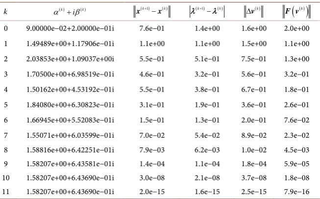
the vector of all ones. Results of numerical experiments are as tabulated in Tables 9-12 respectively. We observed that while it took Algorithm 1 with a fixed complex vector six iterations to converge to the desired eigenvalue

5

1.81999 10× − +2.13950i as shown in Table 9, it took eight, ten and eight

ite-rates for Algorithm 2 (Table 10), Algorithm 3 (Table 11) and Algorithm 4 (Table 12) respectively to achieve the same result. This shows that Algorithm 1 converged faster than the others.

(11)

[image:11.595.209.539.105.240.2]

i

α + β for the 200 by 200 matrix of Example 3.3 using Algorithm 1. Columns 4 and 5 shows that the results converged quadratically for k=1, 2,3 and 4.

k ( )k ( )k

i

α +β ( )k+1 ₋ ( )k

x x _λ( )k+1₋_λ( )k _∆ ( )k

v

( )

( )k F v

0 0.00000e+00+2.50000e+00i 1.0e+00 5.5e−02 1.0e+00 3.8e+01

1 −5.34905e−02+2.48607e+00i 4.2e−02 3.7e−01 3.8e−01 5.5e−02

2 −2.93885e−03+2.11634e+00i 4.0e−03 2.3e−02 2.4e−02 1.6e−02

3 1.47186e−04+2.13954e+00i 4.5e−05 1.3e−04 1.4e−04 9.5e−05

4 1.82101e−05+2.13950e+00i 2.3e−09 1.1e−08 1.1e−08 6.1e−09

[image:11.595.208.540.299.467.2]

5 1.81999e−05+2.13950e+00i 7.9e−15 1.2e−14 1.5e−14 1.8e−14

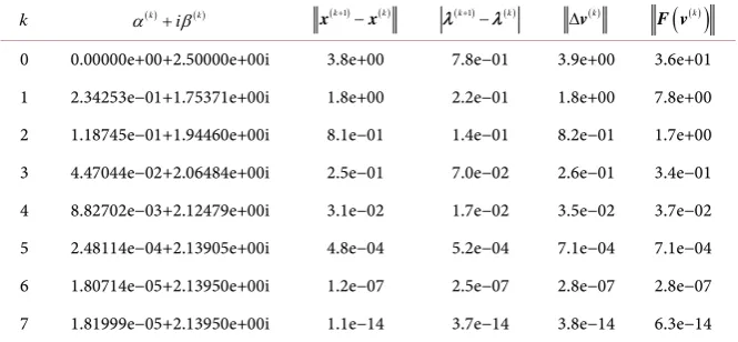
Table 10. Values of _α( )k _and _β( )k _{for the 200 by 200 matrix of Example 3.3 using} Algorithm 2. Columns 6 and 7 show that the results converged quadratically for

3, 4,5,6

k= and 7.

k α( )k β( )k (k+1)₋ ( )k

w w _λ( )k+1 ₋_λ( )k _∆ ( )k

v

( )

( )k

F v

0 0.00000e+00 2.50000 3.8e+00 7.8e−01 3.9e+00 3.6e+01

1 2.34253e−01 1.75371 1.8e+00 2.2e−01 1.8e+00 7.8e+00

2 1.18745e−01 1.94460 8.1e−01 1.4e−01 8.2e−01 1.7e+00

3 4.47044e−02 2.06484 2.5e−01 7.0e−02 2.6e−01 3.4e−01

4 8.82702e−03 2.12479 3.1e−02 1.7e−02 3.5e−02 3.7e−02

5 2.48114e−04 2.13905 4.8e−04 5.2e−04 7.1e−04 7.1e−04

6 1.80714e−05 2.13950 1.2e−07 2.5e−07 2.8e−07 2.8e−07

7 1.81999e−05 2.13950 2.1e−14 2.9e−14 3.6e−14 6.0e−14

Table 11. Values of α( )k _and β( )k _{for the 200 by 200 matrix of Example 3.3 using} Algorithm 3. Columns 6 and 7 show that the results converged quadratically for

3, 4,5,6

k= and 7.

k α( )k β( )k (k+1)₋ ( )k

w w _λ( )k+1 ₋_λ( )k _∆ ( )k

v

( )

( )k

F v

0 0.00000e+00 2.50000 3.8e+00 7.8e−01 3.9e+00 3.6e+01

1 2.34253e−01 1.75371 1.8e+00 2.2e−01 1.8e+00 7.8e+00

2 1.18745e−01 1.94460 8.1e−01 1.4e−01 8.2e−01 1.7e+00

3 4.47044e−02 2.06484 2.5e−01 7.0e−02 2.6e−01 3.4e−01

4 8.82702e−03 2.12479 3.1e−02 1.7e−02 3.5e−02 3.7e−02

5 2.48114e−04 2.13905 4.8e−04 5.2e−04 7.1e−04 7.1e−04

6 1.80714e−05 2.13950 1.2e−07 2.5e−07 2.8e−07 2.8e−07

7 1.81999e−05 2.13950 1.1e−14 9.2e−14 9.2e−14 6.3e−14

8 1.81999e−05 2.13950 1.7e−14 6.8e−14 7.0e−14 5.6e−14

[image:11.595.208.540.527.734.2]

(12)

[image:12.595.207.540.119.273.2]

Table 12. Values of _α( )k _and _β( )k _{for the 200 by 200 matrix of Example 3.3 using} Algorithm 4. Columns 5 and 6 show that the results converged quadratically for

3, 4,5,6

k= and 7.

k ( )k ( )k

i

α +β ( )k+1₋ ( )k

x x _λ( )k+1₋_λ( )k _∆ ( )k

v

( )

( )k

F v

0 0.00000e+00+2.50000e+00i 3.8e+00 7.8e−01 3.9e+00 3.6e+01

1 2.34253e−01+1.75371e+00i 1.8e+00 2.2e−01 1.8e+00 7.8e+00

2 1.18745e−01+1.94460e+00i 8.1e−01 1.4e−01 8.2e−01 1.7e+00

3 4.47044e−02+2.06484e+00i 2.5e−01 7.0e−02 2.6e−01 3.4e−01

4 8.82702e−03+2.12479e+00i 3.1e−02 1.7e−02 3.5e−02 3.7e−02

5 2.48114e−04+2.13905e+00i 4.8e−04 5.2e−04 7.1e−04 7.1e−04

6 1.80714e−05+2.13950e+00i 1.2e−07 2.5e−07 2.8e−07 2.8e−07

7 1.81999e−05+2.13950e+00i 1.1e−14 3.7e−14 3.8e−14 6.3e−14

4. Conclusion

In this paper, we have shown using the ABCD Lemma that the Jacobian ob-tained from adding Ruhe’s normalization to the matrix pencil is non-singular at the root. With a proper choice of the fixed complex vector and an initial guess close to the eigenvalue of interest, we recommend the use of Algorithm 1 for the numerical computation of the desired complex eigenpair of a matrix because of its faster convergence.

Acknowledgements

The authors acknowledge valuable suggestions of an anonymous referee which helped in improving the final version of this paper. The main part of this work was done when the first author was a Ph.D. student at the University of Bath and duly acknowledge financial support in the form of a studentship.

References

[1] Akinola, R.O. and Spence, A. (2014) Two-Norm Normalization for the Matrix Pen-cil: Inverse Iteration with a Complex Shift. International Journal of Innovation in Science and Mathematics, 2, 435-439.

[2] Stewarti, G.W. (2001) Matrix Algorithms, Volume II: Eigensystems. SIAM, Phila-delphia.

[3] Kreyszig, E. (1999) Advanced Engineering Mathematics. John Wiley & Sons Inc., New York.

[4] Ruhe, A. (1973) Algorithms for the Nonlinear Eigenvalue Problem. SIAM Journal on Numerical Analysis, 10, 674-689. https://doi.org/10.1137/0710059

[5] Tisseur, F. (2001) Newton’s Method in Floating Point Arithmetic and Iterative Re-finement of Generalized Eigenvalue Problems. SIAM Journal on Matrix Analysis and Applications, 22, 1038-1057. https://doi.org/10.1137/S0895479899359837

[6] Akinola, R.O. and Spence, A. (2015) Numerical Computation of the Complex Ei-genvalues of a Matrix by Solving a Square System of Equations. Journal of Natural Sciences Research, 5, 144-156.

(13)

Complex Arithmetic. International Journal of Pure & Engineering Mathematics, 3, 137-158.

[8] Keller, H.B. (1977) Numerical Solution of Bifurcation and Nonlinear Eigenvalue Problems. In: Rabinowitz, P., Ed., Applications of Bifurcation Theory, Academic Press, New York, 359-384.

[9] Parlett, B.N. and Saad, Y. (1987) Complex Shift and Invert Strategies for Real Ma-trices. Linear Algebra and Its Applications, 88-89, 575-595.

https://doi.org/10.1016/0024-3795(87)90126-1

[10] Meerbergen, K. and Roose, D. (1996) Matrix Transformations for Computing Rightmost Eigenvalues of Large Sparse Non-Symmetric Eigenvalue Problems. IMA Journal of Numerical Analysis, 16, 297-346.

https://doi.org/10.1093/imanum/16.3.297

[11] Deuflhard, P. (2004) Newton Methods for Nonlinear Problems. Springer, Heidel-berg, 174-175.

[12] Grcar, J. (1989) Operator Coefficient Methods for Linear Equations. Technical Re-port SAND89-8691, Sandia National Laboratories, Albuquerque, New Mexico, Ap-pendix 2.

[13] Nachtigal, N.M., Reichel, L. and Trefethen, L. (1992) A Hybrid GMRES Algorithm for Nonsymmetric Linear Systems. SIAM Journal on Matrix Analysis and Applica-tions, 13, 796-825. https://doi.org/10.1137/0613050

[14] Boisvert, B., Pozo, R., Remington, K., Miller, B. and Lipman, R. Matrix Market.

http://math.nist.gov/MatrixMarket/

Submit or recommend next manuscript to SCIRP and we will provide best service for you:

Accepting pre-submission inquiries through Email, Facebook, LinkedIn, Twitter, etc. A wide selection of journals (inclusive of 9 subjects, more than 200 journals)

Providing 24-hour high-quality service User-friendly online submission system Fair and swift peer-review system

Efficient typesetting and proofreading procedure

Display of the result of downloads and visits, as well as the number of cited articles Maximum dissemination of your research work

Submit your manuscript at: http://papersubmission.scirp.org/