Munich Personal RePEc Archive
Euler Equations for the Estimation of
Dynamic Discrete Choice Structural
Aguirregabiria, Victor and Magesan, Arvind
University of Toronto, University of Calgary
10 April 2013
Online at
https://mpra.ub.uni-muenchen.de/46056/
Euler Equations for the Estimation of
Dynamic Discrete Choice Structural Models
Victor Aguirregabiria
∗University of Toronto
Arvind Magesan
∗University of Calgary
April 8, 2013
Abstract
We derive marginal conditions of optimality (i.e., Euler equations) for a general class of Dynamic Discrete Choice (DDC) structural models. These conditions can be used to estimate structural parameters in these models without having to solve for or approximate value functions. This result extends to discrete choice models theGMM-Euler equation approach proposed by Hansen and Singleton (1982) for the estimation of dynamic continuous decision models. Wefirst show that DDC models can be represented as models of continuous choice where the decision variable is a vector of choice probabilities. We then prove that the marginal conditions of optimality and the envelope conditions required to construct Euler equations are also satisfied in DDC models. The GMM estimation of these Euler equations avoids the curse of dimensionality associated to the computation of value functions and the explicit integration over the space of state variables. We present an empirical application and compare estimates using the GMM-Euler equations method with those from maximum likelihood and two-step methods.
Keywords: Dynamic discrete choice structural models; Euler equations; Choice probabilities.
Corresponding Author: Victor Aguirregabiria. Department of Economics. University of Toronto. 150 St. George Street. Toronto, [email protected]
1
Introduction
The estimation ofDynamic Discrete Choice (DDC) structural models requires the computation of
expectations (value functions) defined as integrals or summations over the space of state variables
of the model. In most empirical applications, the range of variation of the vector of state variables
is continuous or discrete with a very large number of values. In these cases the exact solution of
expectations or value functions is an intractable problem. To deal with this dimensionality problem,
applied researchers use approximation techniques such as discretization, Monte Carlo simulation,
polynomials, sieves, neural networks, etc.1 These approximation techniques are needed not only in
full-solution estimation techniques but also in any two-step or sequential estimation method that
requires the computation of value functions.2 Replacing true expected values with approximations
introduces an approximation error, and this error induces a statistical bias in the estimation of
the parameter of interests. Though there is a rich literature on the asymptotic properties of these
simulation-based estimators,3 little is known about how to measure this approximation-induced
estimation bias for a givenfinite sample.4
In this context, the main contribution of this paper is in the derivation of marginal conditions of
optimality (Euler equations) for a general classDDC models. We show that these Euler equations
provide moment conditions that can be used to estimate structural parameters without solving or
approximating value functions. The estimator based on these Euler equations is not subject to bias induced by the approximation of value functions. Our result extends to discrete choice models
the GMM-Euler equation for dynamic continuous choice models proposed in the seminal work of
Hansen and Singleton (1982). TheGMM-Euler equation approach has been applied extensively to
the estimation of dynamic structural models with continuous decision variables, such as problems
of household consumption, savings, and portfolio choices, or firm investment decisions, among
others. The conventional wisdom was that this method could not be applied to discrete choice
models because, obviously, there are not marginal conditions of optimality with respect to discrete
1
See Rust (1996) and the recent book by Powell (2007) for a survey of numerical approximation methods in the solution of dynamic programming problems. See also Geweke (1996) and Geweke and Keane (2001) for excellent surveys on integration methods in economics and econometrics with particular attention to dynamic structural models. 2The Nested Fixed Point algorithm (NFXP) (Rust, 1987, Wolpin, 1986) is a commonly used full-solution method for the estimation of single-agent dynamic structural models. The Nested Pseudo Likelihood (NPL) method (Aguirre-gabiria and Mira, 2002, 2007) and the method of Mathematical Programming with Equilibrium Constraints (MPEC) (Judd and Su, 2012) are other full-solution methods. Two-step and sequential estimation methods include Condi-tional Choice Probabilities (CCP) (Hotz and Miller, 1993), K-step Pseudo Maximum Likelihood (Aguirregabiria and Mira, 2002, 2007), Asymptotic Least Squares (Pesendorfer and Schmidt-Dengler, 2007), and their simulated-based estimation versions (Hotz et al, 1995, Bajari, Benkard, and Levin, 2007).
3Lerman and Manski (1981), McFadden (1989), and Pakes and Pollard (1989) are seminal works in this literature. See Gourieroux and Monfort (1993, 1997) Hajivassiliou and Ruud (1994), and Stern (1997) for excellent surveys.
choice variables. In this paper, we show that we can represent the dynamic (or static) discrete
choice model as a continuous choice model where the decision variables are choice probabilities
with continuous support. Using this representation of the discrete choice model, we obtain versions
of the marginal conditions of optimality and the Envelope Theorem conditions that we need to
construct Euler equations. Just as in the Hansen-Singleton approach, these Euler equations can be
used to construct moment conditions and to estimate the structural parameters of the model by GMM without having to evaluate/approximate value functions.
Our derivation of Euler equations for DDC models extends previous work by Hotz and Miller
(1993) and Arcidiacono and Miller (2011). Hotz and Miller (1993) show that for DDC models with
an optimal stopping rule structure we can obtain necessary conditions of optimality that involve a
finite (small) number of states, and that moment restrictions based on these conditions can identify
structural parameters in this class of models. Arcidiacono and Miller (2011) extend that result to
a more general class of models with an optimal stopping rule "flavor" such as renewal stopping
problems like the machine replacement model in Rust (1987). In this paper, we derive Euler
equations for a general class of DDC models with the only restrictions being that the unobservables
satisfy the conditions of additive separability in the payofffunction, and conditional independence
in the transition of the state variables.
We present an empirical application where we estimate a model offirm investment. We compare
estimates using the GMM-Euler equations method from those from other methods in the literature,
such as maximum likelihood and sequential estimation methods.
2
Euler equations in dynamic decision models
2.1
Dynamic decision model
Time is discrete and indexed by . Every period, an agent chooses an action within the set of
feasible actions A that, for the moment, can be either a continuous or a discrete choice set. The
agent makes this decision to maximize his expected intertemporal payoffE[P=0−Π(+ +)],
where ∈(01)is the discount factor, is the time horizon that can be finite or infinite, Π() is
the one-period payofffunction at period, and is the vector of state variables at period. These
state variables follow a controlled Markov process, and the transition probability density function
at periodis(+1 | ). By Bellman’s principle of optimality, the sequence of value functions
{() :≥1} can be obtained using the recursive expression:
() = max ∈A
½
Π( ) +
Z
+1(+1)(+1 | ) +1
¾
(1)
The sequence of optimal decision rules {∗() : ≥1} are defined as the argmax in ∈A of the
Suppose that the primitives of the model {Π } can be characterized in terms of vector of
structural parameters. The researcher has panel data for agents (e.g., individuals,firms) over
e
periods of time, with information on agents’ actions and a subset of the state variables. The
estimation problem is to use these data to consistently estimate the vector of parameters. In this
section, we first describe this approach in the context of continuous-choice models, as proposed in
the seminal work by Hansen and Singleton (1982). Second, we show how a general class of discrete choice models can be represented as continuous choice models where the decision variable is a vector
of choice probabilities. Finally, we show that it is possible to construct Euler equations using this
alternative representation of discrete choice models, and that these Euler equations can be used to
construct moment conditions and a GMM estimator of the structural parameters.
2.2
Euler equations in dynamic continuous decision models
Suppose that the decision is a vector of continuous variables in the dimensional Euclidean
space: ∈A⊆ R. The vector of state variables ≡( ) contains both exogenous () and
endogenous () variables. Exogenous state variables, , follow a stochastic process that does not
depend on the agent’s actions{}, e.g., the price of capital in a model offirm investment under the
assumption that firms are price takers in the capital market. In contrast, the evolution over time
of the endogenous state variables,, depends on the agent’s actions, e.g., the stock of capital in a
model offirm investment. More precisely, the transition probability function of the state variables
is:
(+1 | ) = 1{+1=( +1)} (+1 |) (2)
where () is a vector-valued function that represents the transition rule of the endogenous state
variables. Because +1 is an argument of function (), and+1 may include innovation shocks,
this structure of the transition probability allows for a stochastic transition in the endogenous state
variables. It is convenient to represent the transition probability function using the expression in
(2). The following assumption provides sufficient conditions for the derivation of Euler equations
in dynamic continuous decision models.
ASSUMPTION EE-Continuous. (A) The payoff function Π and the transition function () are
continuously differentiable in all their arguments. (B)and are both vectors in the-dimension
Euclidean space and for any value of ( +1) we have that
( +1)
0
=( )
( +1)
0
(3)
where ( ) is a × matrix.
For the derivation of the Euler equations, we consider the following constrained optimization
problem. We want to find the decisions rules at periods and + 1that maximize the
the endogenous state variables +2 conditional on implied by the new decision rules () and
+1()is identical to that distribution under the optimal decision rules of our original DP problem,
∗()and ∗+1(). By construction, this optimization problem depends on payoffs at periods and
+ 1 only, and not on payoffs at + 2 and beyond. And by definition of optimal decision rules,
we have that ∗() and ∗+1() should be the optimal solutions to this constrained optimization
problem. For a given value of the state variables, we can represent this constrained optimization
problem as:
max {+1}∈A2
½
Π( ) +
Z
Π+1(+1 ( +1) +1)(+1 |) +1
¾
subject to: (+1 ( +1) +1 +2) =∗+2( +1 +2)
(4)
where(+1 ( +1) +1 +2) represents the realization of+2 under arbitrary choice
( +1), and ∗+2( +1 +2) is a function that represents the realization of +2 under the
optimal decision rules∗()and∗+1(+1), and it does not depend on( +1). This constrained
optimization problem can be solved using the Lagrangian method. It is possible to show that the
optimal solution should satisfy the following marginal condition of optimality:5
E
µ
Π
0
+ ∙
Π+1
0
+1
−(+1 +1)
Π+1
0
+1
¸
+1
0
= 0 (5)
where E() represents the expectation over the distribution of {+1 +1} conditional on( ).
This system of equations is theEuler equations of the model.
EXAMPLE 1. Optimal consumption and portfolio choice (Hansen and Singleton, 1982). The vector of decision variables is = ( 1 2 ) where represents the individual’s consumption
expenditure, and denotes the number of shares of asset/security that the individual holds in
his portfolio at period. The utility function depends only on consumption, i.e.,Π( ) =().
The consumer’s budget constraint establishes that +P=1 ≤ +P=1, where is
labor earnings, and is the price of asset at time. Given that the budget constraint is satisfied
with equality, we can write the utility function as Π( ) = (− P=1[−−1]), and
the decision problem can be represent in terms of the decision variables (1 2 ). The
vector of exogenous state variables is = ( 1 2 ), and the vector of endogenous
state variables consists of the individual’s asset holdings at −1, = (1−1 2−1 −1).
Therefore, the transition rule of the endogenous state variables is trivial, i.e., +1 =, such that
+10 = 0,+10=I, and the matrix ( ) is a matrix of zeros. Also, given the form
of the utility function, we have thatΠ=−0() and Π−1=0() . Plugging
these expression in the general formula (5), we obtain the following system of Euler equations: for
any asset= 12 :
E¡0()− 0+1(+1) +1 ¢= 0 (6)
2.3
Random Utility Model as a continuous optimization problem
Before we consider Dynamic Discrete Choice models, in this section we describe how a static discrete choice model can be represented as an optimization problem with continuous decision variables in
which standard marginal conditions of optimality are satisfied. Later, we apply this result in our
derivation of Euler equations in Dynamic Discrete Choice models.
Consider the following Additive Random Utility Model, ARUM (McFadden, 1978). The set of
feasible choicesA is discrete and finite and it includes + 1choice alternatives: A={01 }.
Let∈Arepresent the agent’s choice. The payofffunction has the following structure:
Π( ) =() +() (7)
where()is a real valued function, and≡{(0) (1) ()}is a vector of exogenous variables
affecting the agent’s payoff. The vector has a cumulative distribution function (CDF) that
is absolutely continuous with respect to Lebesgue measure, strictly increasing and continuously
differentiable in all its arguments, and with finite means. The agent observes and chooses the
actionthat maximizes his payoff() +(). The optimal decision rule of this model is a function
∗() from the state spaceR+1 into the action spaceA such that: ∗() = arg max
∈A {() +()
}. By the additive separability of the ’s, this optimal decision rule can be written as follows: for
any∈A,
{∗() =} iff {()−()≤()−() for any6=} (8)
Given this form of the optimal decision rule, we can restrict our analysis to decision rules with
the following ‘threshold form: {() =}if and only if{()−()≤()−() for any6=},
where () is an arbitrary real valued function. We can represent decision rules within this class
using a Conditional Choice Probability (CCP) function (), that is the decision rule integrated
over the vector of random variables, i.e.,()≡R1{() =}(). Therefore, we have that
() =
Z
1{()−()≤()−() for any6=} ()
= e(()−() : for any6=),
(9)
where1{}is the indicator function, and e is the CDF of the vector{()−() : for any6=}.
Lemma 1 establishes that in an ARUM we can represent decision rules using a vector of CCPs
P≡{(1),(2), ..., ()} in the-dimension simplex.
LEMMA 1. [McFadden, 1981]. Consider an ARUM where the distribution of is that is
absolutely continuous with respect to Lebesgue measure, strictly increasing and continuously diff
er-entiable in all its arguments. Let ()be a discrete-valued function from R+1intoA={01 };
(2), ..., ()} be a vector in the -dimension simplex S. We can say that (), μe, and P represent the same decision rule in the ARUM if and only if the following conditions hold:
() = P
=0
1{ ()−()≤()−() for any6=} (10)
and for any ∈A,
() =e(()−() : for any6=) (11)
where e is the CDF of the vector {()−() :for any 6=}.
Lemma 2 establishes the invertibility of the relationship between the vector of CCPsPand the
vector of differential payoffs μe.
LEMMA 2. Let Ge()be the vector valued mapping {e1()e2(), ...,e()}from R intoS. Under the conditions of Lemma 1, the mapping Ge() is invertible everywhere. We represent the inverse mapping as e−1().
Given an arbitrary decision rule, represented in terms (), orμ, orP, let Π be the expected
payoffbefore the realization of the vectorif the agent behaves according to this arbitrary decision
rule. By definition,
Π ≡
Z
{ (()) +(()) } () =E( (()) +(()) ) (12)
where the expectation E() is over the distribution of . We can represent this expected payoffas
a function of (), or μ, or P. For our analysis, it is most convenient to represent this expected
payoffas a function of CCPs, i.e.,Π(P). Given its definition, this expected payofffunction can be
written as:
Π(P) =
X
=0
() { () +(P) }
= (0) +(0P) +
X
=1
() {()−(0) +(P)−(0P)}
(13)
where (P) is defined as the expected value of () conditional on alternative being chosen
under decision rule (). That is, (P) ≡ E(() |() =), and as a function of P we have
that
(P) = E³() |()−()≤e−1(P)−e−1(P) for any6=´ (14)
The conditions of the ARUM imply that functions(P)andΠ(P)are continuously differentiable
with respect toPeverywhere on the simplexS. Therefore, this expected payofffunctionΠ(P)has
a maximum on S. We can define P∗ as the vector of CCPs that maximizes this expected payoff
function:
P∗ = arg max
P∈S{ Π
(P)}
Then, we have two representations of the ARUM, and two apparently different decision
prob-lems. On the one hand, we have the discrete choice model with the optimal decision rule ∗()
in equation (8) that maximizes the payoff () +() where once is realized and known to the
agent. We denote this as the ex-post decision problem to emphasize that the decision is after
the realization of is known to the agent. Associated to ∗, we have its corresponding CCP,
that we can represent as P∗, that is equal to Ge(πe) where πe is the vector of differential payoffs
{()e ≡ ()−(0) : for any 6= 0}. For econometric analysis of ARUM, we are interested
in the P∗ representation because these are CCPs from the point of view of the econometrician
(who does not observe ) describing the behavior of an agent who maximizes his payoff given his
knowledge of and . On the other hand, we have the continuous decision problem represented
by equation (15) where the agent chooses the vector of CCPsPto maximize his ex-ante expected
payoffΠ before the realization of. In principle, this second optimization problem is not the one
the ARUM assumes the individual is solving. In the ARUM we assume that the individual makes
his choice after observing the realization of the vector of ’s. Proposition 1 establishes that these
two optimization problems are equivalent, that the choice probabilitiesP∗ and P∗ are the same,
and that P∗ can be described in terms of the marginal conditions of optimality associated to the
continuous optimization problem in (15).
PROPOSITION 1. Let P∗ be the vector of CCPs associated with the optimal decision rule ∗
in the discrete decision problem (8), and let P∗ be the vector of CCPs that solves the continuous
optimization problem (15). Then, (i) the vectors P∗ and P∗ are the same; and (ii) P∗ satisfies
the marginal conditions of optimality Π(P∗)() = 0for any 0, and the marginal expected
payoff Π(P)() has the following form:
Π(P)
() = ()−(0) +(P)−(0P) +
P
=0
()(P()) (16)
Proof in the Appendix.
Proposition 1 establishes a characterization of the optimal decision rule in terms of marginal
conditions of optimality with respect to CCPs. In section 3, we show that these conditions can
be used to construct moment conditions and a two-step estimator of the structural parameters.
Note that the marginal conditions of optimality in equation (16) are with respect to the free
probabilities, i.e., in Π(P), the choice probability for alternative zero should be represented as
1−P=1().
EXAMPLE 2 (Multinomial Logit): Suppose that the unobservable variables () are iid with an
extreme value type 1 distribution. For this distribution, it is possible to show that the function
appendix to chapter 2 in Anderson, de Palma, and Thisse, 1992, for a proof of this result). Plugging
this expression into (16), we get the following marginal condition of optimality:
Π(P∗)
() =()−(0)−ln
∗() + ln∗(0) = 0 (17)
because in this model, for any , the term P=0() [(P)()]is zero.6
EXAMPLE 3 (Binary Probit model): Suppose that the decision model is binary, A = {01},
and (0) and (1) are independently and identically distributed with a normal distribution with
zero mean and variance 2. Let() and Φ() denote the density and the cumulative distribution
functions for the standard normal, respectively, and let Φ−1() be the inverse function ofΦ. Given
this distribution, it is possible to show that: (0 (1)) = √
2
(Φ−1[1−(1)])
1−(1) , and (1 (1)) = √2
(Φ−1[(1)])
(1) . Using these expressions, we have that:7
(0(1))
(1) =
√
2
∙
−Φ−1(1−(1))
1−(1) +
(Φ−1
[(1)]) [1−(1)]2
¸
(1(1))
(1) = √2
∙
−Φ−1((1))
(1) −
(Φ−1[(1)])
(1)2
¸ (18)
Solving these expressions into the first order condition in (16) and taking into account that by
symmetry of the Normal distributionΦ−1(1−(1)) =−Φ−1((1)), we get the following marginal
condition of optimality:
Π(P∗)
(1) = (1)−(0)−
√
2 Φ−1((1)) = 0 (19)
2.4
Euler equations in Dynamic Discrete Choice Models
Consider the dynamic decision model in section 2.1 but suppose now that the set of feasible actions is discrete and finite: A= {01 }. There are two sets of state variables: = (x ), where
x is the vector of state variables observable to the researcher, andrepresents the unobservables
for the researcher. The set of observable state variables x itself is comprised by two types of
state variables, exogenous variables and endogenous variables . They are distinguished by the
fact that the transition probability of the endogenous variables depends on the action, while the
transition probability of the exogenous variables does not depend on. The vector of unobservables
satisfies the assumptions of additive separability (AS) and conditional independence (CI) (Rust,
1994).
6Note that
=0() [(P)()]is equal to() [−1()] +(0) [1(0)] = 0.
7For the derivation of these expressions, it is useful to take into account that0() =− ()andΦ−1
()= 1(Φ−1
Additive Separability (AS): The one-period payoff function is additively separable in the
unobserv-ables: Π( ) =( ) +(),where ≡{() :∈A}is a vector of unobservable random
variables.
Conditional Independence (CI): The transition probability (density) function of the state variables
factors as: (+1|,) = (+1|,) (+1), where () is the CDF of which is
absolutely continuous with respect to Lebesgue measure, strictly increasing and continuously diff er-entiable in all its arguments, and withfinite means.
Under these assumptions the optimal decision rules ∗( ) have the following form:
{∗( ) =} iff {()−()≤( )−( ) for any6=} (20)
where ( ) is the conditional-choice value function that is defined as ( ) ≡ ( )+
R +1
¯
+1(+1) (+1 | ) +1, and ¯() is the integrated value function, ¯() ≡
R
( ) (). Furthermore, the integrated value function satisfies the following integrated
Bellman equation:
¯ () =
Z
max
∈A
½
( ) +() +
Z
¯
+1(+1) (+1| ) +1
¾
() (21)
We can restrict our analysis to decision rules ( ) with the following "threshold" structure:
{( ) =} if and only if {()−() ≤( )−( ) for any 6=}, where( )
is an arbitrary real valued function. As in the ARUM, we can represent decision rules using a
discrete valued function( ), a real valued function ( ), or a probability valued function
(|).
(|) ≡
Z
1{( ) =} ()
= e(( )−( ) : for any6= 0 )
(22)
where e has the same interpretation as in the ARUM, i.e., the CDF of the vector{()−() :
for any 6= }. Lemmas 1 and 2 from the ARUM extend to this DDC model (Proposition 1
in Hotz and Miller, 1993). In particular, at every period , there is a one-to-one relationship
between the vector of value differences μe() ≡ {( )−(0 ): 0} and the vector of
CCPs P() ≡ {( | ): 6= 0}. We represent this mapping as P() = (e μe()), and the
corresponding inverse mapping as μe() =e−1(P()).
Given an arbitrary sequence of decision rules, represented in terms ≡ {() : ≥ 1}, or
e
μ ≡ {μe() : ≥ 1}, or P ≡ {P() : ≥ 1}, let
() be the expected intertemporal payoff
arbitrary sequence of decision rules. By definition,
() ≡ E
µ− P
=0
[+(+(+ +) +) ++(+(+ +))]|
= E
∙
(( ) ) +(( )) +
Z
+1(+1) (+1|( ) )+1
¸
(23)
We denote()as thevaluation function to distinguish it from the optimal value function and to
emphasize that () provides the valuation of any arbitrary decision rule. We are interested in
the representation of this valuation function as a function of CCPs. Therefore, we use the notation
(PP0). Given its definition, this function can be written using the recursive formula:
(PP0) = Π(P) +
Z
+1(+1P+1P0+1) (+1|P) (+1|) +1
(24)
where: Π(P) is the expected one-period profit P=0( | ) [( ) +(P())];
(P()) has the same definition as in the static model, i.e., it is the expected value of ()
conditional on alternativebeing chosen under decision rule ( );8 and (+1|P) is the
transition probability of the endogenous state variablesinduced by the CCP functionP(), i.e.,
P
=0 (|)(+1| ).
The valuation function (PP0) is continuously differentiable with respect to the
choice probabilities over the simplex. Then, we can define P∗ as the sequence of CCP functions
{P∗() : ≥ 1, ∈ X } such that for any ( ) the vector of CCPs P∗() maximizes the values
(PP0) given that future CCPs P0 arefixed at their values in P∗.
P∗() = arg max
P()∈S
©
¡PP∗
0
¢ ª
(25)
As in the ARUM, we have apparently two different optimal CCP functions. We have the CCP
functions associated with the sequence of optimal decision rules∗(), that we represent as{P∗:
≥1}. And we have sequence of CCP functions{P∗ :≥1}defined in equation (25). Proposition
2 establishes that the two sequences of CCPs are the same one, and that these probabilities satisfy
the marginal conditions of optimality associated to the continuous optimization problem in (25).
PROPOSITION 2. Let {P∗
:≥1}be the sequence of CCP functions associated with the sequence
of optimal decision rules {∗ : ≥1} as defined in the DDC problem (20), and let {P∗
: ≥ 1}
be sequence of CCP functions that solves the continuous optimization problem (25). Then, for
every ( ): (i) the vectors P∗
() and P∗() are the same; and (ii) P∗() satisfies the marginal
conditions of optimality
¡P∗P∗
0
¢
(|)
= 0 (26)
8Therefore, we also have that(
P())is equal toE(()|()−()≤−1
(P())−−1
for any 0, and the marginal value has the following form:
(|)
= ( P0)−(0 P0) +(P())−(0P()) +
P
=0
(|)(P(|()))
(27)
where ( P0)is the conditional-choice value function ( )+R +1(+1P+1P0+1)
(+1| ) +1.
Proof in the Appendix.
Proposition 2 shows that we can treat the DDC model as a dynamic continuous optimization problem where optimal choices, in the form of choice probabilities, satisfy marginal conditions
of optimality. Nevertheless, the marginal conditions of optimality in equation (27) involve value
functions. We are looking for conditions of optimality in the spirit of Euler equations that involve
only payofffunctions at two consecutive periods,and+1. To obtain these conditions, we construct
a constrained optimization problem similar to the one for the derivation of Euler equations in section
2.2.
The constrained optimization problem consists offinding the CCP functions at periodsand+1
that maximize the one-period-forward expected profitΠ(P()) + E[Π+1(+1P+1(+1))]
subject to the constraint that the probability distribution of the endogenous state variables +2
conditional on implied by P and P+1 is identical to the distribution of +2 conditional on
under the optimal CCPs of our original periods problem, P∗ and P∗+1. By construction,
this constrained optimization problem depends on payoffs at periods and + 1 only, and not on
payoffs at+ 2and beyond. And by definition of optimality, the CCPsP∗
andP∗+1 should be the
optimal solutions to this constrained optimization problem. Given the structure of our model, the
distribution of +2 conditional on{P()P+1} can written as:
→+2(+2 |PP+1) =
Z
+1(+2 |+1P+1) (+1 |P) (+1|) +1 (28)
where, as defined above,
(|P) is the transition probability of the endogenous state variables
induced by the CCP functionP(), i.e., P
=0 (|) (+1| ).
For a given value of the state variables at period , say , we can represent this constrained
optimization problem as:
max {P()P+1}
∆=
½
Π(P) +
Z
Π+1(+1P+1) (+1|P) +1
¾
subject to: →+2(|PP+1) =
→+2(|P∗P∗+1)
(29)
where → +2(|PP+1) represents the probability distribution of +2 conditional on =
and induced by the CCPs P() and P+1. Suppose that the space of the vector of endogenous
in the constrained optimization problem (29) includes at most|Y|−1restrictions, where|Y|is the
number of points in the support set Y. Therefore, the number of Lagrange multipliers, and the
matrix that we have to invert to get these multipliers is of at most as large as |Y|−1. In fact,
in many models, the number of Lagrange multipliers that we must solve for can be much smaller
than the dimension of the vector of endogenous state variables. This is because in many models
the transition probability of the endogenous state variable is such that, given the state variable at
period , the state variable at period + 2 can take only a limited and small number of possible
values. We present several examples below.
Let Y+() be the set of values that the endogenous state variables can reach with positive
probabilityperiods in the future given that the state today is. To be precise,Y+()includes all
these possible values except one of them because we can represent the probability distribution of+
using the probabilities of each possible value except one. Letλ() ={(+2|) :+2 ∈Y+2()}
be the |Y+2()| ×1 vector of Lagrange multipliers associated to this set of restrictions. The
Lagrangian function for this optimization problem is:
L(P()P+1) = Π(P) + P +1
Π
+1(+1P+1) (+1 |P)(+1|)
− P +2
(+2|) ⎡ ⎣X
+1
+1(+2 |+1P+1) (+1 |P) (+1|) ⎤ ⎦
(30)
Given this Lagrangian function, we can derive the first order conditions of optimality with respect
toP() and P+1 and combine these conditions to obtain Euler equations.
PROPOSITION 3. The marginal conditions for the maximization of the Lagrangian function in
(30) imply the following Euler equations. For every value of :
Π (|)+
X
+1 h
Π+1(+1)−m(+1)0Π
+1(+1)
P+1(+1) i
e
(+1| )(+1|) = 0 (31)
where e(+1| ) ≡ (+1| )−(+1|0 ); Π+1(+1)P+1(+1) is a column vector
with dimension |Y+1()| ×1 that contains the partial derivatives { Π+1(+1 +1) +1(
| +1 +1) } for every action 0 and every value +1 ∈ Y+1() that can be reach from ,
and fixed value for +1; and m(+1) is a |Y+1()| ×1 vector such that m(+1)≡ f+1(+1)0
[Fe+1(+1)0 Fe+1(+1)]−1 Fe+1(+1)0, where f
+1(+1) is the vector of transition probabilities {+1(+2|+1) :+2∈Y+2()}, and Fe+1(+1)is matrix with dimension|Y+1()|×|Y+2()|
that contains the probabilities e+1(+2| +1) for every +2 ∈ Y+2(), every +1 ∈ Y+1(),
and every action 0, with fixed +1.
Proposition 3 shows that in general we can derive marginal conditional of optimality that involve
only payoffs and states at two consecutive periods. The derivation of this Euler equation, described
in the appendix, is based on the combination of the Lagrangian conditions L(|) = 0
and L+1(|+1) = 0. Using the second group of conditions (i.e., L+1(|+1) =
0), we can solve for the vector of Lagrange multipliers as [Fe+1(+1)0 Fe+1(+1)]−1 Fe+1(+1)0 Π+1(+1)P+1(+1), and then we can plug this solution into thefirst Lagrangian conditions,
L(|) = 0. This provides the expression for the Euler equation in (31). The main
com-putational cost in the derivation of this expression comes from inverting the matrices [Fe+1(+1)0
e
F+1(+1)]. The dimension of these matrices is |Y+2()| × |Y+2()|, where Y+2() is the set of
possible values that the endogenous state variable +2 can take given . In most applications,
the number of elements in the set Y+2() is substantially smaller that the whole number of values
in the space of the endogenous state variable, and several orders of magnitude smaller than the
dimension of the complete state space that includes the exogenous state variables. This property
implies very substantial computational savings in the estimation of the model. We now provide
some examples of models where the form of the Euler equations is particularly simple. In these
examples, we have simple closed form expressions for the Lagrange multipliers. These examples correspond to models that are commonly estimated in applications of DDC models.
EXAMPLE 4 (Dynamic binary choice model of entry and exit). Consider a binary decision model,
A={01}, whereis the indicator of being active in a market or in some particular activity. The
endogenous state variableis the lagged value of the decision variable,=−1, and it represents
whether the agent was active at previous period. The vector of state variables is then= ( )
where are exogenous state variables. Suppose that (0) and (1) are extreme value type 1
distributed with dispersion parameter. In this model, the one-period expected payofffunction is
Π( ) =(0|) [(0 ) − ln(0|)]+(1|) [(1 ) − ln(1|)]. The transition
of the endogenous state variable induced by the CCP is the CCP itself, i.e., (+1| ) =
(+1|). Therefore, we can write the ∆function in the constrained optimization problem as:
∆ = Π( ) + P +1
(+1|)£(0|) Π+1(0 +1 +1) +(1|) Π+1(1 +1 +1)¤
(32)
Given , the state variable +2 can take two values, 0 or 1. Therefore, there is only one free
probability in → +2 and one restriction in the Lagrangian problem. This probability is:
→ +2(1| P+1) = P
+1
(+1|) [(0|)+1(1|0 +1) +(1|)+1(1|1 +1)]
(33)
Let()be the Lagrange multiplier for this restriction. For a given, the free probabilities that
enter in the Lagrangian problem are (1|),+1(1|0 +1), and +1(1|1 +1) for any possible
with respect to(1|) is
Π (1|)+
P
+1 £
Π
+1(1)−Π+1(0)−() {+1(1|1 +1)−+1(1|0 +1)}¤(+1|) = 0
(34)
The marginal condition with respect to one of the probabilities +1(1|+1) (for a given value
of +1) is:
Π
+1(0+1+1)
+1(1|0+1) =
Π
+1(1+1+1)
+1(1|1+1) = (). Substituting the marginal condition
with respect to+1(1|+1) into the marginal condition with respect to (1|) we get the Euler
equation:
Π
(1|)+ E
¡
Π+1(1 +1)−Π+1(0 +1) ¢ +
E
³
+1(1|0 +1)
Π
+1(0+1+1)
+1(1|0+1) −+1(1|1 +1)
Π
+1(1+1+1)
+1(1|1+1) ´
= 0
(35)
where we useE()to represent in a compact form the expectation over the distribution of(+1|).
Finally, for the logit version of this model and as shown in Example 2, the marginal expected profit
Π
(1|) is equal to (1 )− (0 )− (ln(1|)− ln(0|)). Taking this into
account and operating in the Euler equation, we can obtain this simpler formula for this Euler
equation: h
(1 )−(0 )− ln
³
(1|) (0|)
´i
+
E
h
(01 +1)−(00 +1)− ln
³
+1(0|1+1)
+1(0|1+1) ´i
= 0
(36)
EXAMPLE 5 (Machine replacement model). Consider a model where the binary choice variable
is the indicator for afirm’s decision to replace an old machine or equipment by a new one. The
endogenous state variableis the age of the "old" machine that takes discrete values{12 }and
it follows the transition rule+1 = 1 + (1−), i.e., if thefirm replaces the machine at period
(i.e., = 1), then at period + 1 it has a brand new machine with +1 = 1, otherwise the firm
continues with the old machine that at+ 1will be one period older. Given , we have that+1
can take only two values,+1 ∈{1 + 1}. Thus, the∆ function is:
∆ = Π() + P +1
(+1|) £(0|) Π+1(+ 1 +1) +(1|) Π+1(1 +1)¤ (37)
Given , we have that +2 can take only three values, +1 ∈ {12 + 1}. There are only two
free probabilities in the distribution of
→+2(+2|). Without loss of generality, we use the
probabilities
→+2(1|)and→+2(2|)to construct the Lagrange function. These probabilities
have the following form:
→+2(1|) = P +1
(+1|) [(0|)+1(1|+ 1 +1) +(1|)+1(1|1 +1)]
→+2(2|) = (1|) P +1
(+1|) +1(0|1 +1)
The Lagrangian function depends on the CCPs (1|), +1(1|1 +1), and +1(1|+ 1 +1).
The Lagrangian optimality condition with respect to(1|) is:
Π (1|) +
P
+1
(+1|)£Π+1(1 +1)−Π+1(+ 1 +1)¤
−(1) P
+1
(+1|) [+1(1|1 +1)−+1(1|+ 1 +1)]
−(2) P
+1
(+1|) +1(0|1 +1) = 0
(39)
And the Lagrangian conditions with respect to +1(1|1 +1) and +1(1|+ 1 +1) are:
Π
+1(1+1)
+1(1|1+1)−(1)+(2) = 0, and
Π
+1(+1+1)
+1(1|+1+1)−(1) = 0, respectively. We can use the
sec-ond set of csec-onditions to solve trivially for the Lagrange multipliers, and then plug in the expression
for this multipliers in the first set of Lagrangian conditions. We obtain the Euler equation:
Π
(1|)+ E
£
Π
+1(1 +1)−Π+1(+ 1 +1)¤
+ E
h Π
+1(1+1)
+1(1|1+1)+1(0|1 +1)−
Π
+1(+1+1)
+1(1|+1+1)+1(0|+ 1 +1) i
= 0
(40)
Finally, taking into account that for the logit specification of the unobservables the marginal
ex-pected profit Π
(1|) is equal to (1 )−(0 )− [ln(1|)−ln(0|)], and
op-erating in the previous expression, it is possible to obtain the following Euler equation:
h
(1 )−(0 )− ln
³
(1|) (0|)
´i
+
E
h
(11 +1)−(1 + 1 +1)− ln
³
+1(1|1+1)
+1(1|+1+1) ´i
= 0
(41)
3
GMM estimation of Euler equations
Suppose that the researcher has panel data of agents over eperiods of time, where he observes
agents’ actions { : = 12 ; = 12 e}, and a subvector of the state variables,
{ : = 12 ; = 12 }. The number of agents is large, and the number of time
periods is typically short. The researcher is interested in using this sample to estimate the structural
parameters of the model,. We describe here the GMM estimation of these structural parameters
using moment restrictions from the Euler equations derived in section 2.
3.1
GMM estimation of Euler equations in continuous decision models
The GMM estimation of the structural parameters is based on the combination of the Euler
equa-tion(s) in (5), the assumption of rational expectations, and some assumptions on the unobservable
state variables. For the unobservables, this literature has considered the following type of
assump-tion.
ASSUMPTION GMM-EE continuous decision. (A) The partial derivatives of the payoff function
are known functions to the researcher up to a vector of parameters , and is a vector of
unob-servables with zero means, not serially correlated, and mean independent of ( −1 −1) such
that E(+1 | +1 ) = 0. (B) the partial derivatives of the transition rule, +10 and
+10, and the matrix ( ) do not depend on unobserved variables: i.e., +10 =
( ),+10 =( ), and ( ) =( ).
Under these conditions, the Euler equation implies the following orthogonality condition in
terms only of observable variables { } and structural parameters : E( ( +1 +1;) |
) = 0, where
( +1 +1;) ≡ ( ;)
+ [(+1 +1;)−(+1 +1;) (+1 +1;) ]( ;)
(42)
The GMM estimator ˆ is defined as the value of that minimizes the criterion function ()0
Ω (), where()≡{1() 2() −1()}is the vector of sample moments
() = 1
P
=1
()( +1 +1;) (43)
and () is a vector of instruments (i.e., known functions of the observable state variables at
period).
3.2
GMM estimation of static random utility models
Consider the ARUM in section 2.3. Now, the deterministic component of the utility function
for agent is ( ;), where is a vector of exogenous characteristics of agent and of the
environment which are observable to the researcher, and is a vector of structural parameters.
Given a random sample of individuals with information on{ }, the marginal conditions of
optimality in equation (16) can be used to construct a semiparametric two-step GMM estimator
of the structural parameters. The first step consists in the nonparametric estimation of the CCPs
(|) ≡ Pr( = | = ). Let Pb ≡ {b(|)} be a vector of nonparametric estimates of
CCPs for any choice alternative and any value of in the sample. For instance,b(|) can be
a kernel (Nadaraya-Watson) estimator of the regression between1{ =} and . In the second
step, the vector of parameters is estimated using the following GMM estimator:
ˆ = arg min
∈Θ
0
³
Pb´ Ω ³Pb´ (44)
where(P)≡{1(P) 2(P) (P)} is the vector of sample moments, with
(P) =
1
P
=1
"
( ;)−(0 ;) +( )−(0 ) +
P
=0
(|)((|))
#
This two-step semiparametric estimator is root-N consistent and asymptotically normal under mild
regularity conditions (see Theorems 8.1 and 8.2 in Newey and McFadden, 1994). The variance
matrix of this estimator can be estimated using the semiparametric method in Newey (1994), or as
recently shown by Ackerberg, Chen, and Hahn (2012) using a computationally simpler
parametric-like method as in Newey (1984).
3.3
GMM estimation of Euler equations in DDC models
The Euler equations that we have derived for DDC model implies the following orthogonality
conditions: E( ( +1; +1 )| ) = 0, where
( +1; +1 ) ≡ Π
(|) +
h
Π+1(+1)−m(+1)0
Π +1(+1)
P+1(+1) i
(+1|) (+1|)
(46)
Note that this orthogonality condition comes from the Euler equation (31) in Proposition 3, but
we have made two changes. First, we have included the expectation E( | ) that replaces the
sumP+1 and the distribution of+1 conditional on( ), i.e., (+1| ) (+1|). And
second, the Euler equation applies to any hypothetical choice,, at period, but in the orthogonality
condition E( ( +1; +1 ) | ) = 0we consider only the actual/observed choice .
Given these conditions, we can construct a consistent an asymptotically normal estimator of
using a semiparametric two-step GMM similar to the one described above for the static model. For
simplicity, suppose that the sample includes only two periods, and + 1. Let Pb and Pb+1
be vectors with the nonparametric estimates of{(|)} and{+1(|+1)}, respectively at any
value ofand +1 observed in the sample. Note that we do not need to estimate CCPs at states
which are not observed in the sample. In the second step, the GMM estimator of is:
ˆ
= arg min ∈Θ
0
³
PbPb+1´ Ω ³PbPb+1´ (47)
where(PP+1) is the vector of sample moments:
(PP+1) =
1
X
=1
( )( +1; +1 ) (48)
( ) is a vector of instruments, i.e., known functions of the observable decision and state
variables at period . As in the case of the static ARUM, this semiparametric two-step GMM
estimator is consistent and asymptotically normal under mild regularity conditions.
4
An Application
This section presents an application of the Euler equations - GMM method to a binary choice model
when to replace an exiting dairy cow by a new heifer. The cow replacement model that we consider
here is an example of asset or "machine" replacement model.9 We estimate this model using data on
dairy cow replacement decisions and milk production using a two step Pseudo Maximum Likelihood
(PML) estimator and the Maximum Likelihood (ML) estimator, and compare these estimates to
those of the Euler equations - GMM method.
4.1
Model
Consider a farmer that produces and sells milk using dairy cows. The farm can be conceptualized
as a plant with a fixed number of stalls , one for each dairy cow. We index time by and stalls
by. In our model, one period of time is a lactation period of13 months. Farmer profits at period
is the sum of profits across the stalls, P=1Π where Π is the profit from stall at period ,
minus the fixed cost of operating a farm with stalls/cows, (). In this application, we take
the size of a farm, , as exogenously given. Furthermore, profits are separable across stalls and we
can view the problem as maximization of profit from an individual stall.
The farmer decides when (after which lactation period) to replace the existing cow by a new
heifer. Let ∈ {01} be the indicator for this replacement decision: = 1 means that the
existing cow is replaced at the end of the current lactation period. The profit from stallat period
is:
Π= ⎧ ⎨ ⎩
( )−() +(0) = 0
( )−()−( ) +(1) = 1
(49)
( ) is the production of milk of the cow in stall at period, where ∈{12 max} is
the current cow’s age or lactation number, and is a cow-stall idiosyncratic productivity. is
the market price of milk. () is the maintenance cost that may depend on the age of the cow.
( ) is the net cost of replacing the existing cow by a new heifer. This net cost is equal to
the market price of a new heifer, , plus some adjustment/transaction costs, minus the market
value of the retired cow. This market value depends on the quality of the meat, and this quality
depends on the age of the retired cow but not on her milk productivity. In what follows we assume
that the prices
and are constants and as such, do not constitute part of the vector of state
variables. So the vector of observable state variables is = ( ) where is the endogenous
state variable, and = is the vector of endogenous state variable.
The estimations that we present below are based on the following specification on the functions
() and (): () = , and () =. That is, the maintenance cost of a cow is linear
in the cow’s age, and the replacement cost isfixed over time.10 While the productivity shock is
9Dynamic structural models of machine replacement have been estimated before by Rust (1987), Sturm (1991), Das (1992), Kennet (1993 and 1994), Rust and Rothwell (1995), Cooper, Haltiwanger and Power (1999), Cho (2002), and Kasahara (2004), among others.
unobservable to the econometrician, as we show below, under some assumptions it can be recovered
by estimation of the milk production function, =( ), where is the amount of milk,
in liters, produced by the cow in stall at period . The transition probability function for the
productivity shock is:
Pr(+1| ) = ⎧ ⎨ ⎩
(+1|) = 0
0(+1) = 1
(50)
An important feature of this transition probability is that the productivity of a new heifer is
independent of the productivity of the retired cow. Once we have recovered , the transition
function for the productivity shock can be identified from the data. The transition rule for the cow
age is trivial: +1 = 1 + (1−) . The unobservables (0) and (1) are assumed iid over
and over with type 1 extreme value distribution with dispersion parameter.
4.2
Data
The dataset comes from Miranda and Schnitkey (1995). It contains information on the replacement
decision, age and milk production of cows from five Ohio dairy farms over the period 1986-1992.
There are 2340 observations from a total of 1103 cows: 103 cows from farmer 1, 187 cows from
farmer 2,365from farmer 3,282from farmer 4, and166cows from the last farmer. The data were
provided by these five farmers through the Dairy Herd Improvement Association.
Here we use the sample of cows which entered in the production process before 1987. The reason for this selection is that for these initial cohorts we have complete lifetime histories for every cow,
while for the later cohorts we have censored durations. Our working sample consists of 357 cows
and 783 observations.
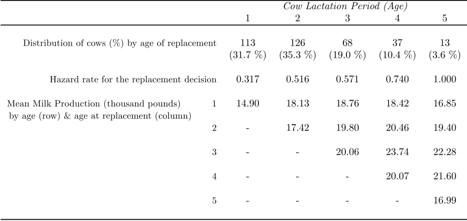
In table 1 we provide some basic descriptive statistics from our working sample. The hazard
rate for the replacement decision increases monotonically with the age of the cow. Average milk
production (per cow and period) presents an inverted-U shape patterns both with respect the
current age of the cow and with respect to the age of the cow at the moment of replacement. This
evidence is consistent with a causal effect of age of milk output but also with a selection effect, i.e.,
more productive cows tend to be replaced at older ages.
Table 1
Descriptive Statistics
(Working sample: 357 cows with complete spells)
Cow Lactation Period (Age)
1 2 3 4 5
Distribution of cows (%) by age of replacement 113 126 68 37 13 (31.7 %) (35.3 %) (19.0 %) (10.4 %) (3.6 %)
Hazard rate for the replacement decision 0.317 0.516 0.571 0.740 1.000 Mean Milk Production (thousand pounds) 1 14.90 18.13 18.76 18.42 16.85
by age (row) & age at replacement (column)
2 - 17.42 19.80 20.46 19.40 3 - - 20.06 23.74 22.28 4 - - - 20.07 21.60
5 - - - - 16.99
4.3
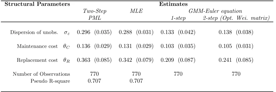
Estimation
In this section we estimate the structural parameters of the profit function using our Euler equations
method, as well as two more standard methods for estimation of dynamic discrete choice models,
the two-step Pseudo Maximum Likelihood (PML) method and Maximum Likelihood (ML) method
for illustrative purposes.
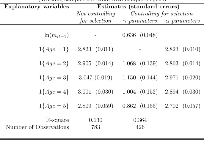
4.3.1 Estimation of Milk Production Function
Regardless of the method we use to estimate the structural parameters in the cost functions, we
first estimate the milk production function, = ( ), outside the dynamic programming
problem. We consider a specification for milk production that is nonparametric in age, and
log-additive in the productivity shock :
ln() = max
P
=1
1{=}+ (51)
A potentially important issue in the estimation of this production function is that we expect age
to be positively correlated with the productivity shock. Less productive cows are replaced at
early ages, and high productivity cows at later ages. Therefore, OLS estimates ofwill not have a
causal interpretation, as the age of the cowis positively correlated with unobserved productivity
. Specifically, we would expect that[|]is increasing in as more productive cows survive