A Binarization Approach for Wafer ID Based on Star-Shape Filter

A Binarization Approach for Wafer ID Based on Star-Shape Filter

Wei-Chih Hsu

1

, Tsan-Ying Yu

2,*,

and Kuan-Liang Chen

1

1

Department of Computer and Communication, National Kaohsiung First University of Science and Technology, Kaohsiung, Taiwan, ROC.

2

Institute of Mechanical and Electro-Mechanical Engineering, National Formosa University, Yunlin, Taiwan, ROC.

Received 15 April 2012; received in revised form 17 May 2012; accepted 22 June 2012

Abstract

The binarization of wafer ID image is one of the key techniques of wafer ID recognition system and its results influence the accuracy of the segmentation of characters and their identification directly. The process of binarization of wafer ID is similar to that of the car license plate characters. However, due to some unique characteristics, such as non-uniform illumination, the unsuccessive strokes of wafer ID, it is more difficult to make of binarization of wafer ID than the car license plate characters. In this paper, a wafer ID recognition scheme based on Star-shape filter is proposed to cope with the serious influence of uneven luminance. The testing results show that our proposed approach is efficient even in situations of overexposure and underexposure the wafer ID with high performance.

Keywords: binarization, wafer ID, star-shape filter, car license plate

1.

Introduction

It is important for Assembly / Test process of semiconductor manufacturing to link to a wafer database by the wafer identification (wafer ID), which is inscribed by a laser scribe system. In order to trace wafer IDs easily, the wafer ID should be recognized automatically. The binarization stage plays an important role in wafer ID recognition.

There are many binarization techniques which can be categorized as global thresholding and local thresholding. Global thresholding [1, 2] selects a single threshold value from the histogram of the entire image. Local thresholding [3, 4] uses localized gray-level information to choose multiple threshold values; each is optimized for a small region in the image. Global threshoding is simpler and easier to implement but its result relies on uniform illumination. It is effective for images with an obviously bimodal histogram and not suitable for images with low contrast. Otsu’s algorithm [5], a conventional global thresholding method, reflects the intensity distribution of an image, but its property of a single threshold results in poor robustness. Local thresholding methods can deal with non-uniform illumination but they are slow. Bernsen algorithm [6] is a typical local threshold technique. It utilizes the extreme of the neighbor to calculate every pixel’s threshold. There are some surveys of various binarization methods reported in the literature [7-9]. More recent studies on this subject can be found [10, 11] .

In this paper, a new image binarization method for wafer ID that we present is a local thresholding method. The binarization of wafer ID recognition is very similar to that of car license plate recognition (LPR). However, because of some

*Corresponding author. E-mail address: [email protected]

wafer ID images’ special features, the binarization scheme must be modified in order to enhance recognition performance. Some special features are described as follows.

Usually, both the brightness and contrast of the wafer ID images are not as sharp as those of the license plate images. There are other disturbances which are caused by non-uniform illumination or poor wafer processes. The wafer scribes are often unsuccessive. Each character is composed of unsuccessive horizontal scribes caused by laser scribe. The unsuccessive wafer scribes will mislead character recognition. Hence, the image binarization stage should take care of it specially.

(1) The spaces between adjacent characters are irregular.

(2) Though the Semiconductor Equipment and Materials International (SEMI) standard is available, the styles of characters will vary as equipments or processes change.

The remainder of this paper is organized as follows. In Section 2, Otsu’s and Bernsen’s methods are briefly reviewed. Section 3 presents the algorithm in detail; Section 4 shows the experimental results. Finally, conclusion and the future work will be addressed.

2.

Two Conventional Binarization Metholds

In this section, we introduce two conventional binarization methods, Otsu’s and Bernsen’s methods, and analyze their limitations when they are applied in the binarization of wafer ID.

2.1. Otsu’s Method

An image is a 2D grayscale intensity function, and contains N pixels with gray levels from 1 to L. The number of pixels with gray level i is denoted fi, giving a probability of gray level i in an image of

N f

p i

i  ₍₁₎

In the case of bi-level thresholding of an image, the pixels are divided into two classes, C1 with gray levels [1, …, t] and

C2 with gray levels [t+1, …, L]. Then, the gray level probability distributions for the two classes are

C1:

₍

₎

,...

₍

t

₎

p

t

p

1 t

1 1





and C2:

₍

₎

,

₍

₎

...

₍

t

₎

,

p

t

p

t

p

2 L

2 2 t

2 1 t







  where







t 1 i

i 1

(

t

)

p



(2)

and



 

 L 1 t

i i

2(t) p

 (3)

Also, the means for classes C1 and C2 are



  t

1

i 1

i

1 _t

ip ) (





(4)







L

1 i 2

i 2

t

ip

)

(





₍₅₎

Let μT be the mean intensity for the whole image. It is easy to show that

2 2 1 1  

  ₍₆₎

1

2 1 

 ₍₇₎

Using discriminant analysis, Otsu defined the between-class variance of the thresholded image as

2 T 2 2 2 T 1 1 2

B  (  )  (  )

     (8)

For bi-level thresholding, Otsu verified that the optimal threshold t* is chosen so that the between-class variance σB2 is

maximized; that is,

)} ( { max

* _t

t 2

B 1 L t

0   

 (9)

When the histogram of wafer ID image has a deep valley, the bottom of the valley is regarded as the threshold to separate the characters from background. But when the image is polluted by noisy, the illumination is poor or the background is complex, the histogram will have more than one deep valley. Then we cannot separate the characters from background correctly by this method.

2.2. Bernsen’s Method

The above original designs are transformed individually into their corresponding generalized chains (kinematic chains). The generalized chain will be involved in various types of members (edges) and joints (vertices, or said kinematic pairs) for all possible assembly in the following steps.

Bernsen’s method is a typical adaptive thresholding method. For each pixel in the image, a threshold has to be calculated. If the pixel value is below the threshold, it is set to the background value, otherwise to the foreground value. An alternative approach to find the local threshold is to calculate the mean of the minimum and maximum values of the local regions. The assumption of this method is that smaller image regions are more likely to have approximately uniform illumination.

The drawback of this method is that it is computational expensive and bring “ghost” phenomena sometimes. The size of the neighborhood must be large enough to cover sufficient foreground and background pixels, otherwise a poor threshold is chosen. Oppositely, choosing too large regions can violate the assumption of approximately uniform illumination.

The Bernsen’s arithmetic can be accomplished by the adaptive threshold operator which maps a given grayscale image F(x,y) into a binary image B(x,y) using a thresholding curved surface T(x,y). We can operate as the following steps:

1. For each pixel in the image, a threshold is calculated.

２

)] , ( min ) , ( max [ ) ,

( ( , ) (, )

y x F y

x F y

x

T xyPxy xyPxy



 (10)

 

 



otherwise 0

y x T y x F 255 y x

B( , ) ( , ) ( , ) ₍₁₁₎

where F(x,y) is the grayscale image, B(x,y) is the binary image, T(x,y) is the thresholding curved surface, Pxy is the

template whose center is (x,y) and size is (2W +1)×(2W +1) , and W is the maximum of estimated stroke width.

3.

The Algotithm of Binarization Approach

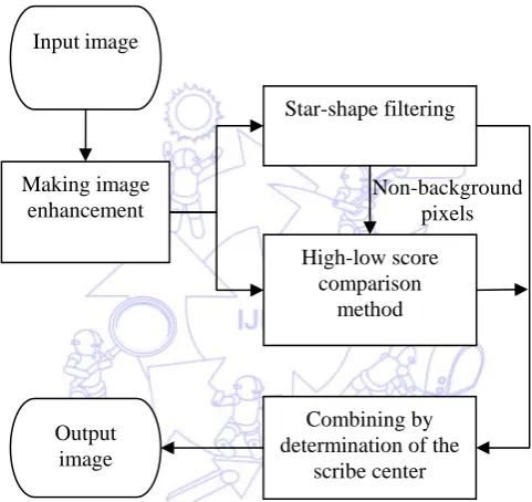
The binarization stage plays an important role in wafer ID recognition. The binarization stage affects the accuracy of character recognition. If a poor binarization algorithm is used, accurate character regions cannot be obtained and the characters cannot be extracted from the wafer ID correctly. While a highly accurate binary image is produced, the character segmentation process will go smoothly and the characters can be obtained from the wafer ID efficiently. The flowchart of our binarization approach is shown in Fig. 1. In the remainder of this paper, the detail of the binarization algorithm will be explored.

Fig. 1 Flowchart of the image binarization algorithm

3.1. Image Enhancement

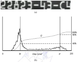
Insufficient exposure, overexposure or uneven luminance will lead to low contrast between the wafer ID string and background. Therefore, we have to examine the contrast of wafer ID image to determine whether to enabled image enhancement or not. First, we analyze the gray level histogram of the wafer ID sub-image. Then, in the gray level histogram, a curve Q denoting the ratio of the accumulated number of pixels of some gray level to total pixels is calculated. We define a gray level br as background reference in which the number of the pixels with gray level less or equal to br is 40% of total pixels. We also define a level sr as stroke reference in which the number of the pixels with gray level greater or equal to sr is 90% of total pixels. One example is depicted in Fig. 2(a)(b). If the difference of the gray level between stroke reference(sr) and background reference(br) is less than δ1, it means that the wafer ID image is low contrast. In other words, we have to enhance

image by enlarging the difference to δ1. The enhancement equation is described in the following:

2 br sr

r  (12)

Input image

Star-shape filtering

High-low score comparison

method

Combining by determination of the

scribe center Output

image Making image

enhancement

) ( )

( 1 _{x r}

br sr r x

f 

 

  (13)

Note that the difference is not allowed to be more than δ1, otherwise the noises will increase after enhancement. The

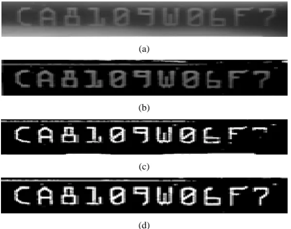
threshold δ1 =25 is determined by experiments. An example of an original and enhanced images are shown in Fig. 3(a)(b). The

low contrast wafer ID images are enhanced obviously.

(a)

(b)

Fig. 2 (a) The cut wafer ID sub-image after locating procedure (b) The gray level histogram and the accumulated ratio curve Q

(a)

(b)

Fig. 3 (a) The original image before enhancement (b) Resulted image after enhancement.

3.2. Image Binarization

Once we have separated the wafer ID string from background, we employ two stages to carry out binarization. At first stage, two methods are applied. The first one called the star-shape filtering will remove luminance disturbance. The second method called the high-low score comparison method which primarily aims to eliminate the noise near wafer scribe edges. At the second stage, we compare and combine the two output images resulted from the star-shape filter and the high-low score comparison method, respectively. At the final stage, the unsuccessive vertical edges are compensated.

3.2.1. The Star-Shape Filtering

scribes usually can be classified into vertical, horizontal, -45 degree, and 45 degree orientation. For the measured pixel, judging from the gray level of the pixels distributing in its corresponding four directions, we can determine whether the measured pixel is foreground pixel or not. Since the scribe width is between 4 and 7 pixels, we set the window size as 99. Let the measured pixel as the window center. We divide the 81 samples of 99 window into upper, lower, left and right regions. For each region, we define its flags whose values are true or false are determined by the following equations:

    _{    } 



_



_ otherwise false 0 y k x f or y x f y k x f if true flag 4 1 k 4 1 k 2 right ) , ( ) , ( ) , (  (14)     _{      } 







 otherwise false 0 k y k x f or y x f k y k x f if true flag 4 1 k 4 1 k 2 right upper ) , ( ) , ( ) , ( _  (15)     _{    } 







 otherwise false 0 k y x f or y x f k y x f if true flag 4 1 k 4 1 k 2 upper ) , ( ) , ( ) , (  (16)     _{      } 







 otherwise false 0 k y k x f or y x f k y k x f if true flag 4 1 k 4 1 k 2 left upper ) , ( ) , ( ) , ( _  (17)     _{    } 







 otherwise false 0 y k x f or y x f y k x f if true flag 4 1 k 4 1 k 2 left ) , ( ) , ( ) , (  (18)     _{      } 







 otherwise false 0 k y k x f or y x f k y k x f if true flag 4 1 k 4 1 k 2 left lower ) , ( ) , ( ) , ( _  (19)     _{    } 







 otherwise false 0 k y x f or y x f k y x f if true flag 4 1 k 4 1 k 2 lower ) , ( ) , ( ) , (  (20)     _{      } 







 otherwise false 0 k y k x f or y x f k y k x f if true flag 4 1 k 4 1 k 2 right lower ) , ( ) , ( ) , ( _  (21)

where f is the image after enhancement, f(x,y) is the measured pixels and δ2 is a threshold, determined as follows.

        otherwise br sr and br sr if 5 3 1 4 2 _     ₍₂₂₎

where sr and br are the stroke and background reference obtained in previous section , and the threshold δ3, δ4 and δ5 are

50, 20 and 15 determined by experiments.

related to flags of flagright, flagupper_righ, flagupper, flagupper_left and flagleft as depicted in Fig. 4(b), the lower region flagleft,

flaglower_left, flaglower_right and flagright as depicted in Fig. 4(c); the left region flagupper, flagupper_left, flagleft, flaglower_left and flaglower

as depicted in Fig. 4(d); the right region flagupper, flagupper_right, flagright, flaglower_right and flaglower as depicted in Fig. 4(e). If any

one of these regions whose related flags are all “true”, then the measured pixel will be set to 0, else the measured pixel will remain the original value. Sometimes, the variance of the gray level near wafer scribe edges is too large, noise can not be removed. The high-low score comparison method is to solve this problem.

Fig. 4 (a) The four distribution orientations of the star-shape filter window (b) The upper region (c) The lower region (d) The left region (e) The right region

3.2.2. The High-Low Score Comparison Method

Assume G(x,y) is the image after the star-shape filtering. Let the HighScoreavg be the average of the gray level of the

pixels which are higher than that of G(x,y) in the window. And let the LowScoreavg be the average of the gray level of the pixels

in the window which are lower than that of G(x,y) in the window. The closer the measured pixels to wafer scribe centers, the higher the values of G(x,y) - LowScoreavgand the lower the values of HighScoreavg - G(x,y)are. In order to separate out the

pixels of the higher gray level from the background, we evaluate and check whether G(x,y) is grater than LowScoreavg +δ8 or

not. Utilizing this criteria, the measured pixels near wafer scribe edges will be classified into wafer ID or background by this method. The method is implemented as follows.

0 ) , ( 0 ) ,

(x y  if G x y 

H ₍₂₃₎        4 4 4

4 ( , ))

(

i j f x i y j Average avg HighScore 0 ) , ( 4 4 4 4 ) , ( ) . (         

 and Gx y

i j j y i x f y x G if ₍₂₄₎        4 4 4

4( , )) (

i j f x i y j Average avg LowScore 0 ) , ( 4 4 4 4 ) , ( ) , (         

 and Gx y

i j j y i x f y x G if ₍₂₅₎

where f is the image after enhancement, G is the image after the star-shape filtering, H is the output image, δ6 the

threshold, (x,y) the measured pixel index. The high-low score comparison method is described as follows:

         otherwise 0 y x

H( , ) 255 ifG(x,y) LowScoreavg 6 G(x,y) (LowScoreavg HighScoreavg)/2, ₍₂₆₎

If G(x,y)> LowScoreavg +δ6 and G(x,y) > (LowScoreavg +HighScoreavg)/2, then the measured pixels are set to 255,

otherwise they are set to 0. The threshold δ6 is set as 15 by experiments.Apply the high-low score comparison method to Fig.

the high-low score comparison method is illustrated in Fig. 5(c).

(a)

(b)

(c)

(d)

Fig. 5 (a)Orginal image (b)Resulted image after star-shape filtering (c) Processing result of the high-low score comparison method (d) Processing result that combined by (b) and (c) and determined by the characteristic of wafer scribe

3.2.3. Combining by Determination of the Scribe Center

The high-low score comparison method aims to deal with those noises which near to wafer scribe edges but not eliminated out by the star-shape filter. As before, the window size is set to 99, and the measured pixel is set at the center.

Since the two images G and H resulting from the star-shape filter and the high-low score comparison method

respectively are not the same for all pixels, we have to combine them in some way. These processing steps are described as follows.

Step 1: If both of them are background pixels in the same position, then the measured pixel is set to 0. If both of them are bright pixels, then the measured pixel is set to 255. Otherwise, its gray level has to be determined in next step by some rules.

Step 2: While we zoom in to observe the cross section of a wafer ID character image, the pixels near the scribe center are brighter than those far away from the scribe center. A typical example of character ‘A’ is shown in Fig. 6(a). Its histogram shown in Fig. 6(b) also reveals the phenomenon. Based on this fact and the phenomenon, the directions of standard wafer scribes can be classified into four types: vertical, horizontal, slope +1 line, slope -1 line. By the star-shape filtering method, reserved pixels have indicated the direction for wafer scribes of G.

0 20 40 60 80 100 120

1 3 5 7 9 11 13 15 17 19 21 23 25 27 29

Fig. 6 (a) The closer the scribe center; the more outstanding the gray levels. The arrows indicate the scribe center (b) The histogram of (a) The locations near to the scribe center have peaks

3.2.4. Unsuccessive Vertical Edge Compensation

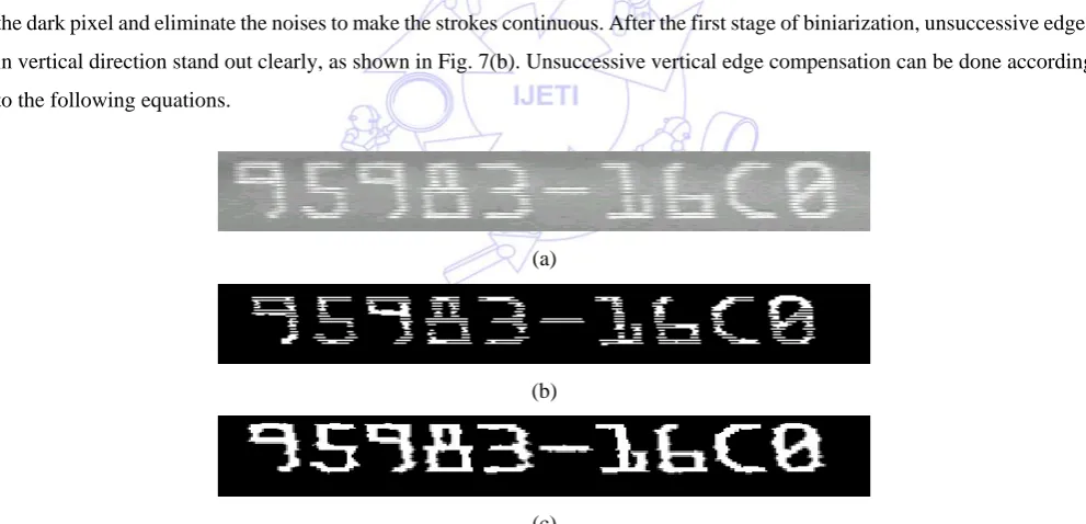
Almost all wafer scribes have unsuccessive edges in vertical direction as depicted in Fig. 7(a). We have to compensate the dark pixel and eliminate the noises to make the strokes continuous. After the first stage of biniarization, unsuccessive edges in vertical direction stand out clearly, as shown in Fig. 7(b). Unsuccessive vertical edge compensation can be done according to the following equations.

(a)

(b)

(c)

Fig. 7 (a) The wafer scribe edges are unsuccessive in the original image. (b) In the processed image, the wafer scribe unsuccessive edges come out clearly. (c) The processing result shows the vertical edges are compensated in the processed image.

where g5 is the image after the scribe center distance determination and 765 comes from 255 times 3. The above equation

  

 _{ }





_

otherwise k j i g if

j i

g _k

0

765 ) , ( 255

) , (

2

2 5

6 (27)

4.

Experimental Results And Analysis

(a)

(b)

(c)

(d)

(e)

(f)

Fig. 8 (a) Orginal wafer ID image (b) The images after enhancement and star-shape filtering The images after high-low score comparing (d) The final binarized images after combining by determination of the scribe center (e) Binarization results by Otsu’s method (f) Binarization results by BernSon’s method

There are several thresholds and parameters in their image processing steps for segmenting out the characters of wafer ID. These parameters may be regarded as system parameters. They are optimized parameters that are obtained from training image data by design of experiment. For example, the masking operation is repeated three times. While training the image data, the first operation is repeated only once, and the result is not sufficient. So, the second operation is repeated twice. The improvement is better than previous step. As the same previous steps, the very little improvement is made after the fifth time operation. Hence, the optimized times for of masking operations is obtained. As the same steps, the other parameters can be optimized.

By analyzing the above results, we can see that the Otsu’s method has serious drawbacks. The left image and the middle image in Fig. 8(a) are normal and overexposure, respectively. Non-uniform illumination will cause the conflict between the object loss and the noise increase. The wafer ID image can not be thresholded effectively. The right image in Fig. 8(a) is underexposure, but uniform illumination will get better performance than the former one. No matter poor or non-uniform illumination, our method can still get more details than Otsu’s method. The object boundaries are much delicate for our method. From Fig. 8, we can directly see that our approach allows to differentiate the characters from the background efficiently.

The result image of Ostu method is quite fuzzy and the characters aren't separated from each other. The one of Bernsen’s method has obvious ghosts and doesn't favor the character recognition. In both of them, character outlines are broken and not clear. By our proposed method, the character stroke is more exquisite.

This is a psycho-visual experiment that is performed to ask a group of people to compare the results of the proposed binarization method with the results obtained by independent binarization techniques. This test is based on ten test Wafer ID images captureed by CCD . For these images we obtain and print the binary images produced by the proposed method and the comparison methods. The printed images were given to 20 persons and asked them to detect visually the best binary image of each image. A percentage of 94% (188/200) of the answers, state that the proposed technique, using the weighting values, result to the best binary image.

With the proposed binarization method, 92% of 125 sample vehicle wafer ID images are correctly recognized. There are 1316 characters in 121 wafer ID images which step in recognition stage successfully. Total 1308 ones are successfully segmented out. The ratio of character recognition is high to 99.39%. The results show that the approach is promising and the binarization rate is close to 100%.

5.

Conclusions

In this paper, a binarization approach based on star-shape filter for wafer ID images is proposed. The proposed approach can effectively enhance the performance of wafer ID recognition. It enhances the wafer ID image at first and original binarization based on star-shape filter and high-low score comparison method are applied in the following. Finally, final binarization result is obtained by combining the determination of the scribe center. Experimental results presented in the paper show that the algorithm provides good results even in situations of uneven luminance, overexposure and underexposure. The experiment results show that the proposed method surpasses Otsu’s method and Bernsen’s method obviously. As a result, we believe that the proposed technique is an attractive alternative to currently available methods for binarizing wafer ID images. We may apply this technique to other applications, such as car license-plate recognition and the container ID numbers recognition.

References

[1] S. H. Shaikh, A. Maiti, and N. Chaki, "Image binarization using iterative partitioning: A global thresholding approach," in Recent Trends in Information Systems (ReTIS), 2011 International Conference, 2011, pp. 281-286.

[2] V. Sokratis, E. Kavallieratou, R. Paredes, and K. Sotiropoulos, "A hybrid binarization technique for document images," Learning Structure and Schemas from Documents, vol. 3163, pp. 165-179, 2011.

[3] S. Cunzhao, X. Baihua, W. Chunheng, and Z. Yang, "Adaptive Graph Cut Based Binarization of Video Text Images," in Document Analysis Systems (DAS), 2012 10th IAPR International Workshop, 2012, pp. 58-62.

[5] H. Chen and R. Gururajan, "Otsu’s Threshold Selection Method Applied in De-noising Heart Sound of the Digital Stethoscope Record," in Advances in Information Technology and Industry Applications, 2012, pp. 239-244. [6] B. Singh, V. Chand, A. Mittal, and D. Ghosh, "A Comparative Study of Different Approaches of Noise Removal for

Document Images," in Proceedings of the International Conference on Soft Computing for Problem Solving (SOCPROS 2011), 2012, pp. 847-854.

[7] P. Stathis, E. Kavallieratou, and N. Papamarkos, "An evaluation survey of binarization algorithms on historical documents," in Pattern Recognition, 2008. ICPR 2008. 19th International Conference, 2008, pp. 1-4.

[8] F. Chun Che and R. Chamchong, "A Review of Evaluation of Optimal Binarization Technique for Character Segmentation in Historical Manuscripts," in Knowledge Discovery and Data Mining, 2010. WKDD '10. Third International Conference on, 2010, pp. 236-240.

[9] M. Sezgin and B. Sankur, "Survey over image thresholding techniques and quantitative performance evaluation," Journal of Electronic Imaging, vol. 13, pp. 146-168, 2004.

[10]T. R. Singh, S. Roy, O. I. Singh, T. Sinam, and K. Singh, "A New Local Adaptive Thresholding Technique in Binarization," International Journal of Computer Science Issues, vol. 8, pp. 271-277, 2011.