Learning Based Falling Detection Using Multiple Doppler Sensors

Learning Based Falling Detection Using Multiple

Doppler Sensors

Shoichiro Tomii, Tomoaki Ohtsuki

Graduate School of Science and Technology, Keio University, Yokohama, Japan Email: [email protected], [email protected]

Received March 9, 2013; revised April 10, 2013; accepted April 17,2013

Copyright © 2013 Shoichiro Tomii, Tomoaki Ohtsuki. This is an open access article distributed under the Creative Commons Attri-bution License, which permits unrestricted use, distriAttri-bution, and reproduction in any medium, provided the original work is properly cited.

ABSTRACT

Automated falling detection is one of the important tasks in this ageing society. Such systems are supposed to have little interference on daily life. Doppler sensors have come to the front as useful devices to detect human activity without using any wearable sensors. The conventional Doppler sensor based falling detection mechanism uses the features of only one sensor. This paper presents falling detection using multiple Doppler sensors. The resulting data from sensors are combined or selected to find out the falling event. The combination method, using three sensors, shows 95.5% ac- curacy of falling detection. Moreover, this method compensates the drawbacks of mono Doppler sensor which encoun- ters problems when detecting movement orthogonal to irradiation directions.

Keywords: Falling Detection; Doppler Sensor; Cepstrum Analysis; SVM; k-NN

1. Introduction

In these days, the elderly population has been growing thanks to advances in the medical field. Healthy, safe and secure life is important particularly for the elderly. How- ever, we are faced with problem of increasing the old-age dependency ratio. The old-age dependency ratio is the ratio of the sum of the population aged 65 years or over to the population aged 20 - 64. The ratio is presented as the number of dependents per 100 persons of working age (20 - 64). According to estimates of the United Na- tions, for about 30 countries, this ratio is projected to reach 30% in 2020 [1]. In particular, it is expected to reach 52% in Japan. There is an urgent need to develop automated health care systems to detect some accidents for the elderly.

Falling detection is one of the most important tasks to prevent the elderly from having crucial accidents. Yu [2] and Hijaz et al. [3] classified falling detection systems

into three groups, wearable device approach, ambient sensors approach, and cameras approach. Wearable de- vices are easy to set up and operate. Devices can be at-tached to chest, waist, armpit, and the back [4]. The shortcomings of these devices are that they are easily broken, and that they are intrusive. Furthermore, the older we become, the more forgetful we become. There- fore, no matter how sophisticated the algorithm imple-

mented on wearable devices is, there is no meaning if they fail to wear them. On the other hand, ambient sen- sors such as pressure and acoustic sensors can also be used. These sensors are cheap and non-intrusive. More- over, they are not prone to privacy issues. However, pressure sensors cannot discern whether pressure is from the user’s weight, while acoustic sensors show high false alarm rate in a situation of loud noise [5]. Cameras en- able remote visual verification, and multiple persons can be monitored using a single setup. However, in private spaces such as bath and restroom, cameras are prohibited. Also in living room, many people do not want to be monitored by cameras.

Doppler sensor is an inexpensive, palm-sized device. It is capable of detecting moving targets like humans. Us- ing this sensor, we can construct passive, non-intrusive, and noise tolerant systems. Activity recognition using Doppler sensor has been actively studied recently. Kim et al. proposed classification of seven different activities

based on micro-Doppler signature characterized by arms and legs with periodic and active motion [7]. Subjects act toward sensor. An accuracy performance above 90% is achieved by using support vector machine (SVM). Tivive

et al. [8] classified three types of motion, free arm-mo-

al. [9] show automatic falling detection. They use two

sensors, which are positioned 1.8 m and 3.7 m away from the point of falling. The data of each sensor is independ- ently processed. Subjects act forward, back, left-side, and right-side fall. The directions of activities include be- tween two sensors, toward a sensor, and away from a sensor.

Doppler sensor is sensitive to the objects moving along irradiation directions; however, less sensitive to movements orthogonal to irradiation directions. For the practical use of Doppler sensors, we propose falling de- tection using multiple Doppler sensors to alleviate the moving direction dependency. By using sensors that have different irradiation directions, each sensor complements less sensitive directions of the other sensors. Sensor data are processed by feature combination or selection meth- ods. In the combination method, features of multiple sensors are simply combined. In the selection method, the sensor is selected based on the power spectral density of the particular bandwidth, which characterizes the fal- ling activity. After the process of each method, features are classified by using SVM or k-nearest neighbors (k- NN). We evaluate both methods in terms of the number of features, the number of sensors, and the type of classi-fier. We also discuss the accuracy of each activity direc-tion and the viability of these methods for the practical use.

The remainder of this paper is organized as follows. In Section 2, we introduce basic Doppler sensor system, how we can determine target velocity from Doppler shift. In Section 3, we explain about flow of the proposed falling detection algorithm using multiple Doppler sen-sors. In Section 4, the sensor setup of the proposed method and the type of tested activities are explained. Our methods are evaluated by comparing them to the one sensor method. We discuss the accuracy of falling detec-tion for each activity direcdetec-tion, and the viability of the proposed feature combination and selection methods in terms of the practical use. In Section 5, we draw conclu- sion.

2. Doppler Sensor

In this section, we discuss the basic information about Doppler sensor. Doppler sensor transmits a continuous wave and receives the reflected wave which has its fre- quency shifted the moving object. The Doppler shift is defined as

2 c d

f

f v

c v



  (1)

where v is the target velocity, c is the light velocity, and fc is the carrier frequency. In Equation (1), sincec v, the target velocity is represented as c



2 d

c

c v

f f

  (2)

fc and c are the given values. Only by observing the Dop-pler shift fd, we can determine the target velocity v.

3. Falling Detection Algorithm Using

Multiple Doppler Sensors

In this section, we show the proposed falling detection algorithm using multiple Doppler sensors. Figure 1 de- picts the algorithm of falling detection. Our approach involves four phases: 1) Decision of extraction time range, 2) Feature extraction, 3) Feature combination/se- lection, 4)Training and classification.

3.1. Decision of Extraction Time Range

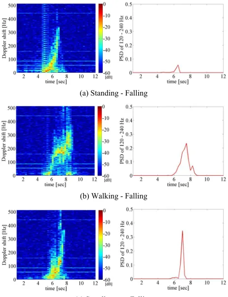
This process is aimed at deciding the timing for extract- ing 4 second features from the voltage data of the sensors. Firstly, we compute spectrogram by using short time Fourier transform (STFT). It is reported that 25 - 50 Hz bandwidth features are suitable to distinguish falling and non-falling when the carrier frequency is 5 GHz [9]. As shown in Equation (2), Doppler shift is proportional to carrier frequency on the condition of the same target ve- locity. Our experiment uses 24 GHz carrier frequency so that bandwidth should be expanded by 4.8 times, i.e. to

within 120 - 240 Hz. On each time bin, which is decided by discrete Fourier transform (DFT) points and window overlap, we calculate the power spectral density (PSD) of 120 - 240 Hz. tmax, the time that the PSD of 120 - 240 Hz becomes maximum in 12 second experiment duration, indicates the time that remarkable event happens. Re- markable events mean activities involving a sudden quick movement using whole body. We specify the 4 second voltage data centered at tmax, and then extract features. Figures 2 and 3 show STFT spectrogram and PSD of 120 - 240 Hz of experienced activities, respectively. Subjects act at about time 7 second.

(a) Standing - Falling

(b) Walking - Falling

(c) Standing up - Falling

Figure 2. Spectrogram (left) and PSD of 120 Hz - 240 Hz (right) of Falling.

3.2. Feature Extraction

Using the 4 second voltage data centered at tmax, we com pute cepstral coefficients. M cepstral coeffi-cients (MFCC) ar -frequency is the

mpresses higher frequency. MFCC is ysis of voice up to about 16 otion, we found empirically

e C0 is direct-

current component. C7-C12 come from latter half of 0 -

10

lled window. The window up

.

a- the selection are compared

- el-frequency

e applied in [9]. Mel

scale definition that emphasizes lower frequency 0 - 1000 Hz and co

basically applied to the anal kHz. On sensing falling m

that up to 500 Hz is enough to observe human activities on condition of 24 GHz carrier frequency. To compute MFCC, 0 - 1000 Hz frequency band is divided into line-arly spaced blocks, which are called filter banks. Sam-pling frequency is 1024 Hz so that there is almost no process to compress higher frequency. Strictly speaking, instead of MFCC, cepstral coefficients analysis is applied. To calculate cepstral coefficients, we use the Auditory Toolbox [10]. The method is as follows.

1) Divide amplitude spectrogram into 13 linearly spaced filter banks.

2) Compute fast Fourier transform (FFT) of amplitude spectrum of each filter bank.

3) Compute discrete cosine transform (DCT) of the obtained data above. The result is called cepstrum.

4) We use C1-C6 coefficients, wher

24 Hz, which is not focused on to observe human activity.

Cepstral coefficient features are computed for each set of 256 DFT points which is ca

date frequency is defined as frame rate. As the frame rate becomes higher, the number of features increases

3.3. Feature Combination/Selection

In our proposal, at most three sensors are used. We em- ploy two methods to make features using multiple Dop- pler sensors, a combination method and a selection method. In the combination method, cepstral coefficients of the sensors are simply associated. Figure 4(a) shows the example of feature structure using two sensors. “l bel” represents the type of activity. In

method, the PSD of 120 - 240 Hz at tmax

among sensors before computing cepstral coefficients.

(a) Walking

(b) Standing – Lying down

(c) Picking up

(d) Sitting on a chair

The sensor that has the largest PSD of 120 - 240 Hz at

tmax is selected for feature extraction. The selected sensor is assumed to catch human motion better than the other sensors.

3.4. Training and Classification

To train and classify the feat res, we use SVM and k-NN For classification by ATLAB, LIBSVM

rnel behaves like RBF with some parameters ifficulty [14] so eneral. Kernel

pillar. A dozen desks ar

Figure 6 shows how multiple sensors are deployed in the proposed methods. The room is rectangular, and its longer side is 10.5 m and shorter side is 7 m. In the mid- dle of the each longer side, there is

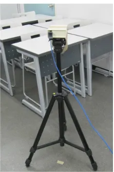
e placed in the rear. The angle between positions X and Y is 135˚, and that between positions Y and Z is 90˚. We used three sensors that transmit continuous wave whose frequency band is 24 GHz. Each sensor uses a slightly different transmit frequency to prevent interference among the sensors. Sampling frequency is 1024 Hz. Sensors are 1 m high from floor as shown in Figure 7, because strength of signal reflected from the torso is higher than that from any other parts of human body, and reflection on the floor cannot be negligible if they are deployed too close to the floor.

u .

using SVM on M

[11] is available. SVM has a kernel function that decides boundaries of groups. As a kernel function, linear, polynomial, radial basis function (RBF), and sigmoid are able to be used on LIBSVM. We exploit the RBF kernel. A linear kernel is the special case of RBF [12], and sigmoid ke

[13]. Polynomial kernel has numerical d that RBF is the most suitable kernel in g

has several parameters and they should be tuned by changing each parameter. When we classify by using k-NN, Euclidean distance between the features is used.

We use four persons (A, B, C, D), who are men from 20’s to 30’s, as training and test subjects as shown in Table 1, and apply cross validation. This process gener- alizes the results of SVM and k-NN. In addition, features are normalized to prevent the greater values from having stronger effect on the results than the others.

4. Performance Evaluation

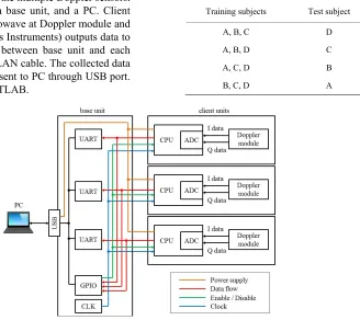
Figure 5 shows contents of the multiple Doppler sensors. They include client units, a base unit, and a PC. Clien

(a) Feature combination method

(b) Feature selection method

Figure 4. Feature structure. Ci is the ith cepstral coefficient. Table 1. Training and testing subject patterns. t

units receive reflected microwave at Doppler module and CPU (MSP430F2618, Texas Instruments) outputs data to base unit. The connection between base unit and each client unit is connected by LAN cable. The collected data of each Doppler sensor are sent to PC through USB port. The data are processed MATLAB.

Training subjects Test subject

A, B, C D

A, B, D C

A, C, D B

B, C, D A

For evaluation of falling detection, subjects took seven activities listed in Table 2. Activities are roughly divided into two categories, “Falling” and “Non-Falling.” Falling includes three following activities.

● Standing-Falling: Keep standing for seconds, then fall down toward each direction at the center, shown as circle in Figure 8.

● Walking-Falling: Walk from a distance of 2.5 m from the center, then fall down at the center.

● Standing up-Falling: Stand up, then fall down to- ward each direction at the center. This simulates lightheadedness.

Non-Falling includes four following activities.

● Walking: Walk from a distance of 2.5 m from the center, across the center, toward each activity direction. Totally 5 m walk.

Figure 6. The deployment of multiple Doppler sensors.

Figure 7. The image of a Doppler sensor.

Standing - Falling Table 2. Falling and Non-Falling activity.

Figure 8. Deployment of multiple sensors.

● Standing-Lying down: Keep standing for seconds, then lie down on the floor toward each direction. ● Picking up: Pick up a pen on the floor. It is put

he center toward activity

● Sitting on a chair: the back of a chair is toward activity direction.

These seven activities are tested in eight directions (A- H) as shown in Figure 8.

The accuracy of falling detection is defined as about 30 cm apart from t

direction.

Accuracy TP TN 100 [%]

TP TN FP FN



 

   (3)

Each variable has the following meaning.

● TP (True Positive): Subject acts falling, and classi-

fied as falling.

● TN (True Negative): Subject acts non-falling, and

classified as non-falling.

● FP (False Positive): Subject acts n n-fal ing, and

clas

FN (False d clas-

sifi

4.1. Frame R

Frame rate is the number of er second. The higher the frame rate be he larger the number of features becomes. Tabl lation be- tween frame cur ling detection. The results of one sensor metho mbination and selection methods using t re shown for comparison.

When we choose k-NN as a classifier, the accuracy increases until frame rate reaches 8 windows/second. When frame rate is higher than 16 windows/second, the degree of increase in accuracy becomes moderate or stable for all methods.

Referring the results using k-NN, we decide to set frame rate at 16 windows/second. We note that frame rate should not be too high because it increases the com- putation load. On the other hand, the low frame rate, which means lack of the features, causes the low accu-

o l

sified as falling.

● Negative): Subjects acts falling, an ed as non-falling.

ate

window updates p comes, t

es 3-5 show the re rate and ac acy of fal

d and the co hree sensors a

Walking - Falling Falling

Standing up - Falling Walking

Standing - Lying down Picking up

Non-Falling

racy bec rs from e problem of high variance in the case of limited sam-

cy

, accuracy does not increase monotoni-

s [13] so that it is generally th

optimum number of features

sh n these

results, we use the optimum frame rate 4 windows/sec- ond on SVM.

Ta racy of fal-

ause the k-NN classifier generally suffe th

pling [15].

When SVM is chosen as a classifier, the best accura for falling detection occurs when the frame rate is 4 windows/second in all the methods. Unlike the case clas-sified by k-NN

cally as frame rate increases. SVM is available to classify linearly non-separable feature

ought to be able to separate complicated features. This result indicates that the

ould be found when SVM is applied. Based o

ble 3. Relation between frame rate and accu ling detection (one sensor method).

Accuracy [%]

k-NN SVM

k = 2 k = 3 k = 4

1 76.8 71.0 73.2 73.2 2 87.1 87.5 87.1 86.6

4 88.

Frame rate _{8 89.3 88.8 88.4}

87.9 90.6 89.3 89.3 [window(s)/second]

8

16 88.8 90.6 89.3 89.3

Table 4. Relation between frame rate and accuracy of fal- ling detection (combination method, three sensors).

Accuracy [%]

k-NN SVM

k = 2 k = 3 k = 4

1 86.6 86.6 88.4 83.5

2 90.2 92.4 93.8 91.5

4 93.8 92.4 93.8 93.3 Frame rate

[window(s)/second]

8 90.6 94.2 94.2 94.1

16 86.6 94.6 93.8 95.5

Table 5. Relation between frame rate and accuracy of fal- ling detection (selsection method, three sensors).

Accuracy [%]

k-NN SVM

k = 2 k = 3 k = 4

1 77.7 83.0 80.4 80.8

2 87.5 87.9 90.2 88.4

4 91.5 90.6 90.2 89.7

8 90.2 90.6 92.4 91.5 Frame rate

[window(s)/second]

16 90.6 90.6 92.4 93.3

4.2. One Sensor Method

Table 6 shows accuracy of falling detection using one nsor. The resul

se t of each sensor is classified by SVM

own in Figure 6, there are three positions, X, Y, and Z. ree sensors, No. 1, 2, and 3. Table 7 show on of each sensor in deployme he result sh n Table 6 is for deployment type i her fferences - curacy based on se or

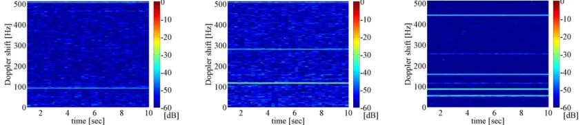
Figures 9-14 sh th wh su

mov olor show stren of PS n dB he s ld be c erized, in principle, lack of partiality of PSD ach ler Ho r, several spectrogra sh tron D i cifi p- ler shift, such as for deployment type ii, position Y (the

nd 440 Hz. To find out the factor of this ix different types of deployments are tested. When comp six types of deploy ent, on eac tion, the str SD occurs on the similar Doppler shift. For nce ositi a strong PSD appea on z D r sh gard of deployment type. o ly, tro D d ot occ of device i rm he effect of

Table 6. Accura of f et us e se

Accuracy [%]

and k-NN. The best accuracy of 90.6 % is achieved on sensor 1 using k-NN (k = 2). As sh

We use th s the positi six nts. T

. T

own i

e are di in ac ns No.

ow e spectrogram en no bject is ing. The c s the

haract

gth D i . T by a pectrogram shou

on e Dopp shift. weve ms ow s g PS n spe c Do p

middle of Figure 10, at 100 Hz, or deployment type iv, position X (the left of Figure 12), at 60, 90, 160, a

strong PSD, s aring ong P

m h posi

insta , in p on Y, rs 100 H opple ift re less Acc rding mpai the s ents, but ng PS by t id n ur because environment.

cy alling d ection ing on nsor.

k-NN Sensor No.

SVM

k = 2 k = 3 k = 4

1 88.8 90.6 89.3 89.3

2 86.6 8 8 8

3 81. 87.

5.3 6.2 5.3

3 86.6 1 86.2

t be pos and r N

Pos

Table 7. Rela ion tween ition senso o. ition

X Y Z

i 1 2 3

ii 1 3 2

iii 2 1 3

iv 2 3 1

v 3 1 2

Deployment type

Figure 9. Spectrogram when no subject is moving in deployment type i. (left: Pos. X, middle: Pos. Y, right: Pos. Z).

Figure 10. Spectrogram when no subject is moving in deployment type ii. (left: Pos. X, m ddle: i Pos. Y, right: Pos. Z).

Figure 11. Spectrogram when no subject is moving in deployment type iii. (left: Pos. X, middle: Pos. Y, right: Pos. Z).

Figure 12. Spectrogram when no subject is moving in deployment type iv. (left: Pos. X, middle: Pos. Y, right: Pos. Z).

Figure 13. Spectrogram when no subject is moving in deployment type v. (left: Pos. X, middle: Pos. Y, right: Pos. Z). I

cular Doppler shift is reported when the Doppler sensor is used through the wall. This appears only on 60 Hz of

non-negligible. On the other hand, the strong PSD on the result of our experiment appears on several Doppler shifts. This means that it is not caused by AC component. It is considered that the strong PSD comes from the re- flection on the wall.

Table 8 shows the accuracy of falling detection for ac- tivity directions. Direction A-H corresponds to 8 direc- tions in Figure 8. The relative position en from each sens

an

rection D relative to sensor 2. Regardless of sensor No., the accuracy decreases in direction orthogonal to irradia- tion direction, that is, directions C and G for sensor 1, directions B and F for sensor 2, and directions D and H for sensor 3. This comes from the characteristics that Doppler sensor can figure out the activity through irra- diation directions. The direction against the sensor also shows low accuracy. It is considered environ- ment

ann

4.3. Feature Combination Method

Table 9 shows the accuracy of falling detection using the combination method. We test with two or three sensors. In particular, when we use two sensors, three types of sensor combinations are tested. In case of two sensors, 92.9% accuracy is achieved when k-NN is used with k set to 4. Just like the result of one sensor method, in Ta- ble 6, accura epends on the position in which the

nd 3 are used, accuracy of falling detection is about 88%. On the other hand, when sensors 1 and 2 are used, an accuracy of 92.9% is achieved using k-NN (k = 4).

By using three sensors, 95.5% accuracy is performed and this is 4.9% higher than the best accuracy of the method using one sensor. In the combination method, three sensors are appropriate for the stable accuracy of falling detection.

Table 11 s s the relation between activity d n 4)

d F, are the

as se _{cy d}

or, in the same row in Table 8, is the same. For in-

ce, direction A relative to sensor 1 is the same as sensor is set. For instance, when sensors 2 and 3, or 1 a st

di

that the how irectio

al noise, which comes from reflection on the wall,

ot be negligible. When the subject moves far from and accuracy of falling detection. We use k-NN (k =as a classifier and deployment type is i in Table 7. As c

the sensor, the strength of microwave, which reflects on

the body, decreases. seen from sensor 1, B and H, C and G, D ansame directions relative to the sensor.

ment type vi. (left: Pos. X, middle: Pos. Y, right: Pos. Z). Figure 14. Spectrogram when no subject is moving in dep

Table 8. Relation between activity directions and

Sensor 1 Sen

loy ac sor

curacy of falling detection (one sensor method).

2 Sensor 3

Direction Accuracy [%] Direction Accuracy [%] Direction Accuracy [%] A 96.4 D 92.9 F 89.3

B, H 96.4 C, E

C, G 75.0 B, F

D, F 94.6 A, G

E 85.7 H

87.5 E, G 87.5

73.2 D, H 80.4

94.6 C, A 89.3

78.6 B 85.7

Table 9. Accuracy of falling detection using the combination method.

Accuracy [%]

k-NN Number of sensors

Table 10. Accuracy of falling detection using the selection method.

Accuracy [%]

k-NN Number of sensors

SVM

k = 2 k = 3 k = 4 SVM

k = 2 k = 3 k = 4

two (sensors 1 & 2) 93.8 92.4 92.4 95.5 two (sensors 1 & 2) 92.0 92.0 92.0 92.9

two (sensors 2 & 3) 92.4 88.8 88.8 88.4 two (sensors 1 & 3) 88.4 91.1 89.7 88.8

three 93.8 94.6 93.8 95.5

two (sensors 2 & 3) 90.2 87.1 87.9 89.7 two (sensors 1 & 3) 89.3 90.6 88.4 91.1

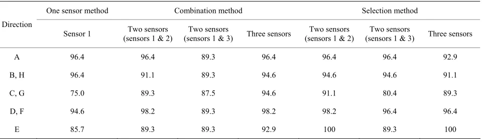
The accuracy of directions C and G in one sensor method is 75.0%. This is 21.4% lower than the direction A, which is the direction that the subject acts toward the sensor. In the combination method using three sensors, the accuracy of directions C and G is 94.6%. This result indicates that the combination method compensates the drawback of Doppler sensor. When using two sensors, the accuracy of directions C and G is im ed compared to t

ends on the deployment. Thus, three sensors are needed for high acc

ency on deploym ur experiment.

4.4. F electio

Table 10 he accuracy of falling detectio sing the selection method. The uracy of falling detectio 5.5%, which o when two sen (1 & 2) are d the featu re classified NN. However s mentioned in t e sensor method d the

ombination method, the difference in accuracy appears

the effect of sensor dependency, we choose three sensor method. Accordingly, th racy in the sel s 93.3%, whic hree sensor me ed N (k = 4).

The relation between activity tion is

sh o red e se eth e

ac dir o ona irra n

di ed. Howeve is st ely low

in co her d s is is cau ed

tion direction, the combination method out- performs the selection method. H may not be alw n practical situation nsider, for example, the case that we are u u sens

one of them is obstructed by en objects such as

fu it ine een t get

an obstructed r c t rec the

D n d t ta oti he

features of the combination method are constructed using features obtained from all the sensors. Thus, the obstructed sensor produces features that are different from the training data. This means that the system that simply combines the features is not tolerant to a situation that the sensors are obstructed by some objects.

Alternatively, the selection method has an advantage in the situati at a part of the sensors is obstructed. me objects, the selection method excludes the data of the

of which or to choose is based on the sel of the largest D of 120 - 240 Hz at t . Th the obstructed

se the data vironme are

no ta moving around hus, the PSD o - 240 Hz b es smaller than that of the senso is not obstr . Therefore, th ion method i re suit- able for practical use.

4.5. True Positive Rate and False Positive Rate

When analyzing systems of falling detection, true posi- rate (FPR) are often

prov on th

hat of one sensor method. However, the accuracy de- Even if one of the multiple sensors is obstructed by so p

uracy of falling detection and less depend- obstructed sensor. This is because the decision ent in o

eature S n Method

shows t n u

highest acc

n is 9 ccurs sors

used, an res a by

k-, a he on an

c

in the feature selection methods using two sensors. To alleviate

e best accu h is in the t ection methods i

thod and classifi by k-N

direc and accuracy own in Table 11. C mpa to on nsor m od, th curacy in the ection rthog l to diatio rection is improv

mp n with th

r, it ill relativ ariso gorit e ot ect fe irection e fro . Th ly on s nsor. by the al hm to sel atur m on e se

In the view of the robustness in the direction orthogonal to irradia

owever, that

ays the case i s. Co

sing m fall

ltiple ors, and

rniture or plants. W hout l of sight betw he tar d the sensor, the senso anno eive oppler informatio relate o the rget m on. T

sens PS

ection e data of max

in the en

nsor is like nt that there

rgets . T f 120

ecom r that

ucted e select s mo

tive rate (TPR) and false positive

used. TPR and FPR are calculated as follows.

,

TP FP

TPR FPR

TP FN FP TN

 

  (4)

when FN becomes 0, TPR is equal to 1. Considering that FN is critical on falling detection system, TPR should be

near 1. On the other hand, FPR should be near 0 because FP indicates over care. However, there sometimes exists

trade-off between TPR and FPR. For practical systems, it

is ideal that TPR reaches 1 and FPR reaches 0.

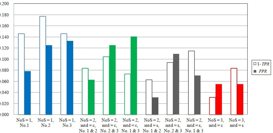
Figure 15 shows FPR and 1-TPR in each method.

Both values should be near 0. Abbreviations “NoS,” “mtd = s,” and “mtd = c” in this figure means “Number of sensors,” “method = selection,” and “method = combina- tion,” respectively. Comparing to the conventional me- thod using individual Doppler sensor data, in the pro- posed method using multiple Doppler sensor data, FPR

and 1-TPR decrease.

ect od Table 11. Relation between activity dir One sensor method Combination meth

ions and accuracy of falling detection. Selection method Direction

Sensor 1 _{(sensors 1 & 2)} Two sensors _{(sensors 1 & 3)}Two sensors Three sensors _{(sensors 1 & 2)}Two sensors _{(sensors 1 & 3)} Two sensors Three sensors

A 96.4 96.4 89.3 96.4 96.4 96.4 92.9

B, H 96.4 91.1 89.3

C, G 75.0 89.3 87.5

D, F 94.6 98.2 89.3

E 85.7 89.3

94.6 94.6 94.6 91.1

94.6 91.1 80.4 89.3

98.2 98.2 96.4 96.4

d True positive rate on e

Figure 15. Results of False positive rate an ach method.

. Conclusion

This paper pro detection us Doppler sen e the combinat

t ds to e ures. ati

achieves 95.5% accuracy of fa

(k = . In this m , three sens re used. D er

sens s are less sen e to the di orthogon the irradiation di than the o directions

ev e combin method co sates this draw- ba oppler r and shows gh accu n eac rection. T e achieves % accuracy using k-NN (k = 4). In th ethod, three

sen-sors e used. Thi so improves the accuracy of the direction orthogonal to the irradiation direction. However, the accuracy of the direction is still relatively low compared to the other directions. Although the se- lection method does not outperform the combination method in the view of the robustness of activity direction, we consider the idea of selection method to be useful for the practical use. The selection method excludes data of the echoless sensor such as accidentally obstructed by furniture or plants. Our future work is to construct the hybrid method between the combination and selection method.

REFERENCES

[1] Department of Economic and Social Affairs, “Population Division: World Population Prospects: The 2010 Revi- sion,” United Nations,Department of Economic and So- cial Affairs, 2011.

[2] X. Yu, “Approaches and Principles of Fall Detection for Elderly Andpatien

tional Conference

[3] F. Hijaz, N. Afzal, T. Ahmad and O. Hasan, “Survey of Fall Detectionand Daily ng Techniques,” Proceedings of International Conference on Information

er gie kist e

[4] Noury, A. , P. Rume . Bourke, G ghin, V. Rialle and J. Lundy, “Fall Detection-Principles and thods,” Proceedings of the Annual International ence of th E EMBS, P 2007, 1663-1666

[5] erry, S. Kellog, S. Vaidya, Youn, H. d H. Sharif, “Surveyand Evaluation of Real-Time Fall Detec- n Approach Proceeding the 6th Int ional Symposium of HONET, Egypt, 28-30 December 2009, pp. 158-164.

[6] S. Ram, C. Christianson, Y. Kim and H. Ling, “Simula- tion and Analysis of Human Micro-Dopplers in through- Wall Environments,” IEEE Transactions on Geoscience and Remote Sensing, Vol. 48, No. 4, 2010, pp. 2015-2023.

doi:10.1109/TGRS.2009.2037219

5

poses falling sors. We propos

ing multiple ion and selec- ion metho xtract feat The combin on method lling detection using k-NN 4)

or

ethod sitiv

ors a rection

oppl al to rection ther . How- er, th

ck of D

ation senso

mpen

the hi racy i h di he selection m thod 93.3

is m ar s method al

t,” Proceedings of the 10th Interna- of the IEEE HealthCom, Singapore,

7-9 July 2008, pp. 42-47.

Activity Monitori

and Em

2010, pp. 1-6. ging Technolo s, ICIET, Pa an, 14-16 Jun

N. Fleury au, A . Lai

Me 29th

Confer pp.

e IEE

. aris, 22-26 August

J. P J. H. Ali an

tio es,” s of ernat

[7] Y. Kim and H. Ling, “Human Activity Classification Based on Microdopplersignatures Using a Support Vector Machine,” IEEE Transactions on Geoscience and Remote Sensing, Vol. 47, No. 5, 2009, pp. 1328-1337.

doi:10.1109/TGRS.2009.2012849

[8] F. Tivive, A. Bouzerdoum and M. Amin, “Automatic Human Motion Classification from Doppler Spectro- grams,” Proceedings of the 2nd International Workshop of CIP, Elba Island, 14-16 June 2010, pp. 237-242. [9] L. Liu, M. Popescu, M. Skubic, M. Rantz, T. Yardibi and

P. Cuddihy, “Automatic Fall Detection Based on Doppler Radar Motion Signature,” Proceedings of the 5th Interna- tional Conference of Pervasive Health, Dublin, 23-26 May 2011, pp. 222-225.

https://engineering.purdue.edu/~malcolm/interval/1998-0 covery, Vol. 2, No. 2, 1998, pp. 121-167.

009715923555 10/

[11] C. Chang and C. Lin, “LIBSVM: A Library for Support Vector Machines.”

http://www.csie.ntu.edu.tw/~cjlin/libsvm/

[12] S. S. Keerthi and C.-J. Lin, “Asymptotic Behaviors of Support Vector Machines with Gaussian Kernel,” MIT Press Journals, Vol. 15, No. 7, 2003, pp. 1667-1689. [13] C. J. Burges, “A Tutorial on Support Vector Machines for

Pattern Recognition,” Data Mining and Knowledge Dis-

doi:10.1023/A:1

Recognition,” Proceedings of the IEEE Con-[14] V. N. Vapnik, “The Nature of Statistical Learning The-

ory,” 2nd Edition, Springer, New York, 1999.

[15] H. Zhang, A. Berg, M. Maire and J. Malik, “SVM-KNN: Discriminative Nearest Neighbor Classification for Visual Category