Abstract—An explicit method based on the central difference method for nonlinear transient dynamic analysis of spatial beams with finite rotations using corotational total Lagrangian finite element formulation is presented. The kinematics of the beam element is described in the current element coordinate system constructed at the current configuration of the beam element. The beam element has two nodes with six degrees of freedom per node. Three rotation parameters referred to the current element coordinates are defined to determine the orientation of element cross section. A rotation vector is used to represent the finite rotation of a base coordinate system rigidly tied to each node of the discretized structure. Note that the values of nodal rotation vectors are reset to zero at current configuration. The element deformation nodal forces and inertia nodal forces are systematically derived by consistent linearization of the fully geometrically nonlinear beam theory, the d'Alembert principle and the virtual work principle in the current element coordinates. The standard central difference method is applied to the incremental displacement and rotational vector, and their time derivatives. The orientation of the end cross section of the beam element is updated by the incremental nodal rotation vector. A Numerical example is presented to demonstrate the accuracy and efficiency of the proposed method.
Index Terms—Corotational total Lagrangian formulation, Dynamics, Explicit time integration, Geometrical nonlinearity.
I. INTRODUCTION
HE implicit methods based on the Newmark direct integration method have been extensively employed in nonlinear transient dynamic analyses of beam structures undergoing large displacements and finite rotations (e.g. [1- 4]). In [3], a corotational total Lagrangian finite element formulation for the nonlinear dynamic analysis of spatial elastic Euler beam using consistent linearization of the geometrically non-linear beam theory was presented. The standard Newmark method was applied to the incremental displacement and rotational vectors, and their time derivatives. The formulation was proven to be very effective
Manuscript received February 26, 2015.
Chu Chang Huang is with Department of Mechanical Engineering, National Chiao Tung University, 1001 Ta Hsueh Road, Hsinchu, 300, Taiwan (e-mail: [email protected]).
Wen Yi Lin is with Department of Mechanical Engineering, De Lin Institute of Technology, 1 Alley 380, Ching Yun Road, Tucheng, Taiwan (e-mail: [email protected]).
Fumio Fujii is with Department of Mechanical Engineering, Gifu University,Gifu 501-1193, Japan (e-mail: [email protected]).
Kuo Mo Hsiao is with Department of Mechanical Engineering, National Chiao Tung University, 1001 Ta Hsueh Road, Hsinchu, 300, Taiwan (phone: 886-3-5712121-55107; fax: 886-3-5720634; e-mail: [email protected]).
by numerical examples studied in [3]. However, the application of the explicit method in the nonlinear dynamic analysis of three-dimensional beams with finite rotations has been rather limited (e.g. [5, 6]). The object of this paper is to present an explicit method based on the central difference method for nonlinear transient dynamic analysis of spatial beams with finite rotations using corotational total Lagrangian finite element formulation.
The element description is based on the corotational total Lagrangian formulation described previously in [3, 7, 8]. In this formulation, each dement is associated with a Cartesian coordinate system constructed at the current configuration of the beam element. The element coordinate system is just a local coordinate system updated at current configuration of the beam element, not a moving coordinate system. Thus, the velocity and acceleration defined in the element coordinate system are absolute velocity and acceleration. For the purpose of treating arbitrarily large rotation of node in space, the orientation of the node is described by a base coordinate system rigidly tied to each node of the discretized structure. A nodal rotation vector [7] is used to represent the finite rotation of the base coordinate system. In this study, the values of nodal rotation vectors are reset to zero at current configuration, thus, the values of the first and second time derivative of the nodal rotation vector are equal the values of the spatial nodal angular velocity and acceleration [3].
The element deformation and inertia nodal forces are systematically derived by using the d'Alembert principle and the virtual work principle. A numerical procedure of explicit method based on the central difference method is proposed here for the solution of the nonlinear equations of motion. A numerical example is presented and compared with the results obtained using the Newmark method to demonstrate the accuracy and efficiency of the proposed method.
II. FINITE ELEMENT FORMULATION
The element developed here has two nodes with six degrees of freedom per node. The kinematics of the beam element and the corotational total Lagrangian finite element formulation proposed in [3, 7, 8] are adapted and employed here. In the following only a brief description of the beam element is given.
A. Basic Assumptions
The following assumptions are made in derivation of the beam element behavior: (1) The beam is prismatic and slender, and the Euler-Bernoulli hypothesis is valid. (2) The cross section of the beam is doubly symmetric. (3) The unit extension of the centroid axis of the beam element is uniform. (4) The cross section of the beam element does not deform in
An Explicit Method for Geometrically Nonlinear
Dynamic Analysis of Spatial Beams
Chu Chang Huang, Wen Yi Lin, Fumio Fujii, and Kuo Mo Hsiao
its own plane and strains within this cross section can be neglected.
B. Coordinate Systems
In order to describe the system, we define three sets of right handed rectangular Cartesian coordinate systems:
1. A fixed global set of coordinates, XiG (i = 1, 2, 3) (see Fig. 1); the nodal coordinates, displacements, rotations, velocities, and accelerations, and the equations of motions of the system are defined in this coordinates.
2. Element cross section coordinates, xiS (i = 1, 2, 3) (see Fig. 1); a set of element cross section coordinates is associated with each cross section of the beam element. The origin of this coordinate system is rigidly tied to the centroid of the cross section. The x1S axis is chosen to coincide with the normal of the unwrapped cross section and the x2S and
S
x3 axes are chosen to be the principal directions of the cross section.
3. Element coordinates, xi (i = 1, 2, 3) (see Fig. 1); a set of element coordinates is associated with each element, which is constructed at the current configuration of the beam element. The origin of this coordinate system is located at node 1, and the x1 axis is chosen to pass through two end nodes of the element; the x2 and x3 axes are determined by the method proposed in [7]. Note that this coordinate system is just a local coordinate system not a moving coordinate system. The deformations, deformation nodal forces, inertia nodal forces, and mass matrix of the element are defined in terms of these coordinates.
C. Kinematics of Beam Element
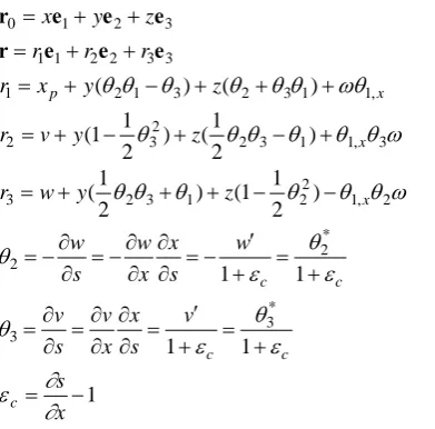
In this study only the doubly symmetric cross section is considered. Let Q (Fig. 1) be an arbitrary point in the beam element, and P be the point corresponding to Q on the centroid axis. The position vector of point Q in the undeformed and deformed configurations referred to the element coordinates may be expressed as [8]:
3 2 1
0 e e e
r x y z (1)
3 3 2 2 1
1e e e
rr r r (2)
x
p y z
x
r1 (213) (231)1,
2 3 1 1, 3 2
3
2 )
2 1 ( ) 2 1 1
( z x
y v
r
2 1, 2
2 1
3 2
3 )
2 1 1 ( ) 2
1
( z x
y w
r
c c
w s x x w s w
1 1
* 2
2 (3)
c c
v s x x v s v
1 1
* 3
3 (4)
1
x s c
(5)
where xpxp(x,t),vv(x,t) andww(x,t) are the x1, 2
x and x3 coordinates of point P, respectively, in the
deformed configuration, 11(x,t) and 1,x1,x(x,t)are the twist angle and twist rate of the deformed centroid axis, respectively, (y,z) is the Saint Venant warping function for a prismatic beam of the same cross section, s is the arc length of the centroid axis, and cis the unit extension of the centroid axis. The orientation of element cross section is determined byi (i = 1, 2, 3), thus, i are called rotation parameters [7, 8]. Here, the lateral deflections of the centroid axis, v and w are assumed to be the cubic Hermitian polynomials of x, and the rotation about the centroid axis, 1, is assumed to be the linear polynomials of x.
The relationship among xp , v, andw, and x may be given as [8]
dx w v u
x x
x
x c p
2 1 2 , 0
2 , 2
1 [(1 ) ]
(6)where u1 is the displacement of node 1 in the x1 direction. Note that due to the definition of the element coordinate system, the value of u1 is equal to zero. However, the variation and time derivatives of u1 are not zero. The axial displacements of the centroid axis, u(x,t)xp(x,t)x may be determined from the lateral deflections and the unit extension of the centroid axis using (6).
Making use of the assumption of uniform unit extension, c
of the centroid axis may be calculated using (6) and the current chord length of the beam element.
D. Element Nodal Force Vector, and Mass Matrix
The element deformation nodal forces and inertia nodal forces are systematically derived by consistent linearization of the fully geometrically nonlinear beam theory, the d'Alembert principle and the virtual work principle in the current element coordinates.
The virtual work principle requires that
qtf qtf qtf
(7)
z y
Q
P S x3
S x2
x
w
v
S
x
2 Sx
12
u
)
0
,
0
,
(
l
s
1
x
2x
P
x
3
x
1
P S x3
P
Fig. 1. Coordinate system.
G
X1
G
X2
G
[image:2.595.306.537.213.415.2] [image:2.595.49.245.546.739.2]
V t V(1111 21212 21313)dV rrdV
} , , ,
{ 1 1 2 2
q u u (8)
} , , ,
{ 1 1 2 2
q u u (9)
} , , ,
{ 2 *2
* 1
1 θ u θ
u
q
(10)
} , , ,
{1 1 2 2
f f f m f m
f D I
(11) }
, , ,
{1 1 2 2
f f f m f m
f D I
(12)
} , , ,
{1 1 2 2
f f f m f m
f D I
(13)
) 1 ( 2 1
, ,
11 x
t xr
r
, y
t x , , 12
2 1
r r
. .
2 1
, ,
13 z
t xr
r
(14)
where j = 1, 2, uj {uj,vj,wj} denote the virtual displacement vectors at nodes j, j {1j,2j,3j}
denote vectors of virtual spatial rotation at nodes j, }
, ,
{ 1j 2j 3j j
denote the corresponding virtual variation of rotation vectors j {1j,2j,3j} at nodes j, and θ*j {1*j,2*j,3*j} {1j,wj,vj} denote the corresponding virtual variation of { , , 3* }
* 2 * 1 *
j j j j θ
} , ,
{ 1j wj vj
{1j,(1c)2j,(1c)3j} at nodes j.
f (,,), are generalized element internal nodal force vectors conjugate to q, { 1 , 2 , 3 }
j j j j f f f
f ( ,, ) are nodal force vectors corresponding to uj and
} , , { 1 2 3
j j j j m m m
m ( ,, ) are generalized nodal moments corresponding to j , j and
* j
θ
, respectively. fD and fI ( ,,) are deformation nodal force vectors and inertia nodal force vectors corresponding to
V(1111 21212 21313)dV and
V tdV
r r
,
respectively. V is the volume of the undeformed beam element, 1j (j = 1, 2, 3) are the variation of the Green strain 1j in (14) corresponding to q. 1j (j = 1, 2, 3) are the second Piola-Kirchhoff stress. For linear elastic material,11E11, and 1j 2G1j (j = 2, 3), where E is Young’s modulus and G is the shear modulus. is the density, r and r are the variation and the second time derivative of r in (2), respectively. Note that the element coordinate system is just a local coordinate system not a moving coordinate system, thus r is the absolute acceleration. The higher order terms of nodal parameters in the element nodal forces are neglected by consistent second order linearization in this study. Note that the values of rotation parameters i (i = 1, 2, 3) will converge to zero, and their time derivatives i and i will converge to constants with the decrease of the element size. Thus, the coupling between rotation parameters and their time derivatives are not considered in this study.
Note that ij are infinitesimal rotations about the xi
axes, thus mij are moments about the xi axes at element local nodes j, respectively, and mj is a vector quantity. ij are not infinitesimal rotations about the xi axes, thus, mij are not moments about the xi axes at nodes j and
j
m is not a vector quantity. However, the values of the rotation vectors at nodes j, j are reset to zero at the current configuration
of the structure in this study. Thus, the values of j are
equal tothe values of the corresponding j, and the values
of jand j are equal to the values of the corresponding
angular velocity vectors ωj and angular acceleration
vectorsω j at nodes j, respectively [3]. The values of mj, j
, and j are therefore equal to the values of the corresponding mj, ωj, andω j, respectively, so the rules
of vector addition also apply to the addition of mj, j, and
j
in this study. * ij
are not infinitesimal spatial rotations about the xi axes, thus
ij
m are not conventional moments. The values of mij are not equal to the values of corresponding mij, because the values of
* ij
are not equal to the values of corresponding ij at deformed state [3, 7], so the rules of vector addition can not apply to the addition of
j
m *
j
θ , and θ*j.
Here, the global nodal parameters of the system are chosen to be the components of nodal displacement vector and nodal rotation vector referred to the global coordinates. To assemble the element equations into the global equations, the element nodal parameters and element nodal forces should be consistent with the global nodal parameters and global nodal forces. Therefore q and fare chosen to be the element nodal displacement vector and the element nodal force vector.
q and f can be transformed from element coordinate system to the global coordinate system using the standard procedure of vector transformation.
The relation between q and q may be expressed as [3, 8]
q T q (15)
q is related to q through the same relationships that exists between qand q [3], i.e.:
T q
q (16)
The time derivative of (16) may be expressed by
T q T q
In view of (7) and (15), the relation between fand f may be expressed as
T f
f t
(18) where f may be calculated using (2-7) and (14). For
convenience, f are divided into four vectors fi (i = a, b, c,
d) and expressed as } , { 11 12
I f f
a D a
a f f
f (19)
} , , ,
{ 21 31 22 32
I f m f m
b D b
b f f
f
} , , ,
{ 31 21 32 22
I f m f m
c D c
c f f
f
} , { 11 12
I m m
d D d
d f f
f
) 2 3 (1
[ c c
D
a AE
f (20)
1 1 ] 2 2 2 ) ( 2 , 2 , 2 ,1 v dx
L EI dx w L EI dx L I I E xx z xx y x z y
EI vxxdxb z D
b N ,
f
EI wxxdx c y D
c N ,
f
GJ EIp c d xdx EKI d xdx
D d 3 , 1 , 1 2 1 ) (
N N
f Iv a a a I
a m u f
f (21)
a t a a a A N N dxu
m
} , {u1 u2 a
u
v w dx v w dxdx
L x
A x x x
L
x x a
Iv
a [ ( ) 0( ) ]
2 , 2 , 0 2 , 2 , N f Iv b b b I
b m u f
f
A dx Iz b btdx
t b b
b N N N N
m
} , , , {v1 v1 v2 v2 b
u
Iz b cvxdx Iz b wxdx
Iv
b 2 N , 2 N1,
f Iv c c c I
c m u f
f
A dx Iy c ctdx
t c c
c N N N N
m
} , , ,
{w1 w1 w2 w2 c
u
Iy c cwxdx Iy c vxdx
Iv
c 2 N , 2 N1,
f Iv d d d I
d m u f
f
I I dx I d dtdx
t d d z y
d N N N N
m ( ) }
, {11 12
d
u
Iy Iz dvxwxdx
Iv
d ( ) N , ,
f
dA z Iy
2
, Iz
y dA 2, I
2dA (22)
z y dA
J {( y) ( z) }
2 , 2
,
, KI
y z dA 2 2 2) (
in which the range of integration for the integral
()dx is from 0 to L, A is the cross section area, Nk (k = a, d) are shape functions of elementary bar element,Nk (k = b, c) areshape functions of elementary beam element and
/dx d() )
( . mi (i = a, b, c, d) are consistent mass matrices, and fiIv (i = a, b, c, d) are vectors of velocity coupling terms of element inertia nodal forces.
In view of (21), element inertia nodal force vector fI may be expressed by
Iv I
mq f
f (23)
where m is the element mass matrix assembled by the submatrices given in (21).
If the coupling between rotation parameters i (i = 1, 2, 3) and their time derivatives are not considered, from (16), (17) and (23), one may obtain
Iv I
mq f
f (24)
Iv Iv
mT q f
f (25)
E. Equations of Motion
The nonlinear equations of motion may be expressed by vI
D
t F F
P Q
M () (26)
where M is the mass matrix, Q is the second time derivative of the vector of global nodal parameters Q, P(t) is the external nodal force vector, FDis the deformation nodal force vector, and FvI is the inertia nodal force vector corresponding to the velocity coupling terms of the element inertia nodal force.
M, FvI and FD are assembled from the element mass matrix, element nodal force vectors, which are calculated using (17)- (25) first in the current element coordinates and then transformed from element coordinate system to global coordinate system before assemblage using standard procedure.
III. NUMERICAL PROCEDURE
An incremental method based on the central difference method (CDM) is proposed here for the solution of the nonlinear equations of motion. The basic steps involved in the numerical solution of (26) are outlined as follows. Let t
denote the time step size, and time tn tn1t (n1). Let 1
n
Q , Qn1, and Qn1 denote the vector of global nodal parameters, velocity, and acceleration of the structure at time
1 n
t (n1), respectively, and
1
1
n n
n Q Q
Q
nodes j and time tn(n1).
Let Qn1, Qn, Qn1, Qn1, Qn1, SG ij
n1e denote the known values at time tn(n1). The values of Qn1, Qn,
n
Q and Qn , SG ij
ne may be obtained by the following incremental procedure.
(a) Extract Gj , the global incremental nodal rotation vector corresponding to each element local nodes j (j = 1, 2) from Qn1 for each element. Extract
G j
u , the global nodal displacement vector corresponding to each element local nodes j (j = 1, 2) from Qn for each element. Determine
SG ij
ne by application G
j
to n1eSGij . Then determine the current element coordinates, element deformation nodal parameters ij and unit extension c for each element using
SG ij ne ,
G j
u , and the method described in [3, 7, 8]. Then, calculate the element deformation nodal force vectors using (18), (20), and assemble structural deformation nodal force vector FnD.
(b) Reset the values of the elements in Qncorresponding
to nodal rotation vectors to zero.
(c) Extract the global nodal velocity vector corresponding to each element from Qn1 (or backward difference QbnQn1/t), and then transform them to the current element coordinates using standard procedure. Then calculate time derivative of element nodal rotation parameters using (16) and (17). Then calculate element inertia nodal force vector fIv using (21) and (25). Then, transform fIv from the current element coordinates to the global coordinates using standard procedure to assemble
vI n
F .
(d) Transform the element mass matrices from the current element coordinates to the global coordinates using a standard procedure. Then assemble the structural mass matrix M using the element mass matrices.
(e) Calculate Qnusing
vI n D n n
n P F F
Q
M ((26)). (f) Let Qn Qn t Qn
2 1
,Qn1QnQn, and t
n n
n(Q Q 1)/2
Q .
When n1, Qn1Q0 and Qn1Q0 can be obtained from the initial conditions, and Qn1Q0 can be calculated using (26); Q1is calculated by
0 2
0 0 1
2 Q
Q Q
Q t t .
IV. NUMERICAL STUDIES
The example studied is a clamped beam subjected to a central eccentric concentrated load as shown in Fig. 2. The load history is also shown in Fig. 2. The geometry of the beam and the material properties are L0.508m ,
m
b0.0254 , h3.175103m , Young's modulus
GPa
E207 , Poisson’s ratio 0.3 , and density 3
/ 2713kg m
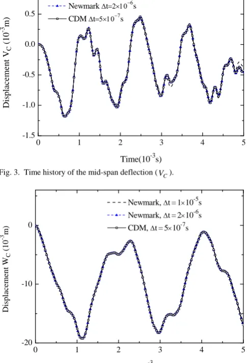
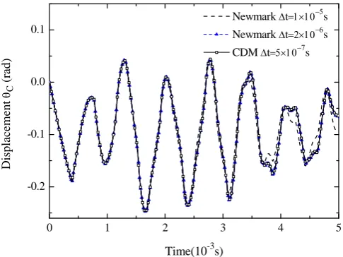
. The eccentricity of the concentrated load is e6103 m. Because of symmetry, only one-half of the beam is modeled by 15 elements. Figures 3 - 5 show a comparison between the time histories of the mid-span deflections and axial rotation obtained by the present method (CDM) and by the Newmark method [3]. The time steps
s 10 5 . 0 6
t
is used for the present method, and
s 10 1 5
[image:5.595.310.542.202.350.2]t and 2106s are used for the Newmark method. Very good agreement between these two results can be observed.
Fig. 2. Clamped beam subjected to concentrated load.
[image:5.595.306.549.397.754.2]Fig. 3. Time history of the mid-span deflection (VC).
Fig. 4. Time history of the mid-span deflection (WC).
L
C D
A B
F
history Load
) ( ) (t N F
2844
) (s t
S
X3
b h
e
F
S
X2
C D
Mid cross U X1G,
V XG2, W X3G,
0 1 2 3 4 5
-1.5 -1.0 -0.5 0.0 0.5 1.0
D
isp
lacemen
t V
C
(1
0
-3 m)
Time(10-3s)
Newmark ts Newmark ts CDM ts
0 1 2 3 4 5
-20 -10 0
Newmark, t=110-5s Newmark, t=210-6s CDM, t=510-7s
Di
splac
eme
n
t W
C
(1
0
-3 m)
Fig. 5. Time history of the mid-span rotation (C).
V. CONCLUSIONS
An explicit method based on the central difference method for nonlinear transient dynamic analysis of spatial beams with finite rotations using corotational total Lagrangian finite element formulation is presented. The global nodal parameters of the system are chosen to be the components of nodal displacement vector and nodal rotation vector. The values of the nodal rotation vectors are reset to zero at the current configuration of the structure in this study. The standard central difference method is applied to the incremental displacement and rotational vector, and their time derivatives. The orientations of the nodes are updated by the incremental nodal rotational vectors. The element coordinate system constructed at the current configuration of the beam element is just a local inertial coordinate system not a moving coordinate system, thus the first and second time derivatives of the position vector of the beam element defined in the element coordinates are the absolute velocity and acceleration. The beam element developed has two nodes with six degrees of freedom per node. Three rotation parameters referred to the current element coordinates are defined to determine the orientation of element cross section. Both the element inertia and deformation nodal forces are systematically derived by using consistent second order linearization of the fully geometrically nonlinear beam theory, the d'Alembert principle and the virtual work principle. The values of rotation parameters will converge to zero, and their time derivatives will converge to constants with the decrease of the element size, thus, the coupling between rotation parameters and their time derivatives are not considered in this study. The formulation is intended for explicit integration procedures, so stiffness matrices are not developed. The element equations are constructed first in the element coordinate system and then transformed to the global coordinate system by using standard procedure. The standard central difference method is applied to the incremental displacement and rotational vector, and their time derivatives.
From the numerical example studied, the accuracy and efficiency of the proposed method are well demonstrated.
It is believed that the corotational total Lagrangian
formulation of the beam element and the numerical procedure of the explicit method presented here may represent a valuable engineering tool for the dynamic analysis of spatial beam structures.
REFERENCES
[1] A. Cardona and M. Geradin, A beam finite element non-linear theory with finite rotation, Internat. J. Numer. Meths. Engrg., Vol. 26, 1988, pp. 2403-2438.
[2] J.C. Simo and L. Vu-Quoc, On the dynamics in space of rods undergoing large motions- a geometrically exact approach, Comput. Methods Appl. Mech. Engrg., Vol. 66, 1988, pp. 125-161.
[3] K. M. Hsiao, J. Y. Lin and W. Y. Lin, A Consistent Co-Rotational Finite Element Formulation for Geometrically Nonlinear Dynamic Analysis of 3-D Beams, Comput. Methods Appl. Mech. Engrg., Vol. 169, 1999, pp. 1-18.
[4] T. N. Le, J. M. Battini and M. Hjiaj, Dynamics of 3D beam elements in a corotational context: a comparative study of established and new formulation, Finite Elements in Analysis and Design, Vol. 61, 2012, pp. 97–111.
[5] T. Belytschko and B. J. Hsieh, Nonlinear transient finite element analysis with convected coordinates, Internat. J. Numer. Meths. Engrg , Vol. 7, 1973, pp. 255-271.
[6] T. Belytschko and L. Schwer, Large displacement, transient analysis of space frames, Internat. J. Numer. Meths. Engrg., Vol. 11, 1977, pp. 65-84.
[7] K. M. Hsiao, A Co-rotational Total Lagrangian Formulation for Three Dimensional Beam Element, AIAA Journal, Vol. 30, 1992, pp. 797- 804.
[8] W. Y. Lin and K. M. Hsiao, Co-Rotational Formulation for Geometric Nonlinear analysis of Doubly Symmetric Thin-Walled Beams, Comput. Methods Appl. Mech. Engrg., Vol. 190, 2001, pp. 6023-6052.
0 1 2 3 4 5
-0.2 -0.1 0.0 0.1
Newmark ts Newmark ts CDM ts
D
isp
lacemen
t
C
(r
ad)