Remarks on Direct System Identification Using
Hypercomplex–Valued Neural Network with
Application to Time–Series Estimation
Kazuhiko Takahashi, Junpei Ozaki, Yasunao Nakahara, Yuka Wakaume,
Takahiro Hirayama, and Masafumi Hashimoto
Abstract—This study discusses a design method for system identification using multilayer hypercomplex–valued neural net-works, such as complex, hyperbolic, bicomplex and quaternion neural networks, and investigates its characteristics. The di-rect transfer function identifier, which employs a multilayer hypercomplex–valued neural network, is used to estimate the output of the target system. A computational experiment involv-ing estimation of a discrete–time dynamic plant is conducted to evaluate the feasibility of the hypercomplex–valued neural network–based direct transfer function identifier. As a practical application of dynamic system identification, the direct transfer function identifier is used to estimate historical foreign exchange data and motion data ofTaijiquanin addition to investigating its characteristics. The experimental results show the effectiveness of the proposed direct transfer function identifier.
Index Terms—Hypercomplex–valued neural network, System identification, Dynamic systems, Historical data, Motion data.
I. INTRODUCTION
T
HE use of hypercomplex numbers for neural networks has attracted increasing attention from engineering re-search fields because it helps to learn to handle a wide variety of geometric objects and their transformation in the form of hypercomplex numbers. To overcome classically hard–to– treat intractable problems with real–number neural networks, high–dimensional neural networks based on hypercomplex numbers, such as complex numbers and quaternions, have been investigated [1] and their effectiveness in solving mul-tidimensional problems has been demonstrated [2]. Complex neural networks have been used successfully in various engineering applications, for example, filtering, time–series signal processing, communications, image processing and video processing [3]. As an extension of complex numbers, quaternions decrease computational complexity significantly in three– or four–dimensional problems compared to real numbers. Therefore, quaternion neural networks can cope with multidimensional issues more efficiently by directly employing quaternions. Several studies have used quaternion neural networks in applications requiring multidimensional signal processing, for instance, rigid body attitude control [4], colour image processing [5], signal processing [6][7], filtering [8], pattern classification [9] and inverse problems [10]. In previous studies, we have presented control schemes for robot manipulators [11] and servo–controllers [12][13].Manuscript received December 8, 2016; revised December 20, 2016. K. Takahashi, J. Ozaki, Y. Nakahara, Y. Wakaume and T. Hi-rayama are with Information Systems Design, Doshisha University, Ky-oto, Japan e-mail: {katakaha@mail, bun1063@mail4, bum1040@mail4, bun1084@mail4, bun1016@mail4}.doshisha.ac.jp.
M. Hashimoto is with Intelligent Information Engineering and Science, Doshisha University, Kyoto, Japan e-mail: [email protected].
In this study, a method of system identification based on a hypercomplex–valued neural network is discussed from the viewpoint of its applicability to time–series signal processing of dynamic systems. A method of designing a direct transfer function identifier in which the neural network output serves as an estimate of the output of a target system is presented. Computational experiments for estimating the output of a discrete–time dynamic plant, historical foreign exchange data and motion data of Taijiquan movements are conducted to evaluate the feasibility of the proposed neural network–based direct transfer function identifier.
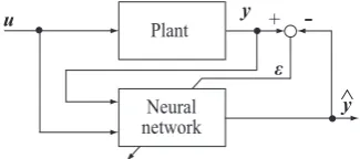
II. DIRECTTRANSFERFUNCTIONIDENTIFIER BASED ON HYPERCOMPLEX–VALUEDNEURALNETWORKS Figure 1 shows a schematic of a direct transfer function identifier using a neural network, where the output of the neural network converges with the plant output after the neural network is trained and the plant transfer functions are composed in the neural network. Here y ∈ Rq is the
plant output,u ∈Rp is the input to the plant and yˆ ∈Rq
is the output of the identifier that consists of the output from the hypercomplex–valued neural network. Assuming a multilayer network topology that has one input layer, one output layer andN hidden layers (N ≥0), the input–output relationship of the hypercomplex–valued neural network is defined. Because all signals, weights and thresholds of a hypercomplex–valued neural network are hypercomplex numbers, the algebra of hypercomplex numbers should be followed to derive a training algorithm for hypercomplex– valued neural networks. In this study, complex, hyperbolic, bicomplex and quaternion numbers are considered so as to consist of the neural networks.
Complex numbers consist of two real numbers and an imaginary unit:C:={z =z0+z1i|z0, z1∈R,i2 =−1}. The sum of two complex numbersz1 andz2 is given as
z1±z2= (z10±z20) + (z11±z21)i,
Plant
y Neural
network
y +
-u
ε
[image:1.595.344.507.678.750.2]^
while the product of two complex numbers is given as
z1z2= (z10z20−z11z21) + (z10z21+z11z20)i. The norm of a complex number is defined as
|z|=√zz∗=
√
z2
0+z21,
wherez∗=z0−z1iis the conjugate of the complex number z.
Hyperbolic numbers consist of two complex numbers and an imaginary unit:D:={z=z0+z1h|z0, z1∈R,h2= 1}. The sum of two hyperbolic numbers z1 andz2 is given as
z1±z2= (z10±z20) + (z11±z21)h,
while the product of two hyperbolic numbers is given as
z1z2= (z10z20+z11z21) + (z10z21+z11z20)h. The norm of a hyperbolic number is defined as
|z|=√zz∗=
√ |z2
0−z21|,
where z∗ = z0 −z1h is the conjugate of the hyperbolic numberz.
Bicomplex numbers consist of two complex numbers and an imaginary unit, that is four real numbers and three imaginary units: T := {z = z1+z2i2|z1,z2 ∈ C,i22 =
−1}={z=z0+z1i1+z2i2+z3h|z0, z1, z2, z3∈R,i21= i22 = −1,i1i2 = h,h2 = 1}. The sum of two bicomplex numbers z1 andz2 is given as
z1±z2= (z10±z20) + (z11±z21)i1
+(z12±z22)i2+ (z13±z23)h, while the product of two bicomplex numbers is given as
z1z2= (z10z20−z11z21−z12z22+z13s2h)
+(z11z20+z10z21−z13z22−z12z23)i1
+(z12z20−z13z21+z10z22−z11z23)i2
+(z13z20+z12z21+z11z22+z10z23)h. The norm of a bicomplex number is defined as
|z|=
√
zz†+z?(z†)?
2 =
√
z2
0+z21+z22+z23, wherez?=z
0−z1i1+z2i2−z3h,z∗=z0+z1i1−z2i2−
z3handz†=z0−z1i1−z2i2+z3hare the conjugates of the bicomplex number z.
Quaternion numbers consist of four real numbers and three imaginary units: H := {z = z0 +z1i+ z2j+
z3k|z0, z1, z2, z3 ∈ R,i2 = j2 = k2 = ijk = −1,ij =
−ji=k,jk=−kj=i,ki=−ik=j}. The sum of two quaternion numbersz1 andz2 is given as
z1±z2= (z10±z20) + (z11±z21)i
+(z12±z22)j+ (z13±z23)k, while the product of two quaternion numbers is given as
z1z2= (z10z20−z11z21−z12z22−z13z23)
+(z11z20+z10z21−z13z22+z12z23)i
+(z12z20+z13z21+z10z22−z11z23)j
+(z13z20−z12z21+z11z22+z10z23)k.
The norm of a quaternion number is defined as
|z|=√zz∗=
√
z2
0+z21+z22+z23,
wherez∗ = z0−z1i−z2j−z3k is the conjugate of the quaternion numberz.
The output of them-th neuron unit in then-th layerx(mn)
is defined as follows:
x(mn)=fm(v
(n)
m )
v(mn)= ∑
l
wml(n)xl(n−1)+φ(mn) , (1)
where w(mln) is the weight between the l-th neuron unit in the (n−1)-th layer and the m-th neuron unit in the n-th layer, φ(mn) is the threshold of the m-th neuron unit in the n-th layer, andf(·) is an activation function of the neuron unit. Here the activation function requires analyticity of the function in the hypercomplex number domain [14].
The hypercomplex–valued neural network is trained to minimize the cost function J defined by the norm of the output error(t)as follows:
J(t) = 1
2
∑
σ ∑
k
|k(t)|2, (2)
wherek(t) =dk−x
(o)
k (t),dk is the desired output of the k-th neuron unit in the output layer and the superscriptnof o indicates the output layer and t is the iteration number. Assuming increment of the network parameters in the t -th iteration ∆ω(t) = ω(t+ 1)−ω(t) where the vector ω(t) is composed of network parameters such as weights and thresholds, variation of the cost function ∆J can be calculated as follows:
∆J = J(t+ 1)−J(t)
≈ (
∂J(t)
∂ω(t)
)T
∆ω(t) +
(
∂J(t)
∂ω∗(t)
)T
∆ω∗(t).
Setting∆ω(t) =−η ∂J(t)
∂ω∗(t) and∆ω
∗(t) =−η∂J(t)
∂ω(t)yields ∆J = −2η∂J(t)
∂ω(t)
2≤0,
where the factor η is positive. Increment of the parameters in the output layer is given as
∆w(kjo)(t) =η∑ σ
δk(t)x∗
(n−1)
j (t)
∆φ(ko)(t) =η∑ σ
δk(t)
, (3)
whereδk(t) =k(t)f0k(v
(o)
k (t)), and the superscript (n−1)
indicates the hidden layer links to the output layer, while increment of the parameters in the hidden layer is given by
∆w(jin)(t) =η∑ σ
δj(t)x∗
(n−1)
i (t)
∆φ(jn)(t) =η∑ σ
δj(t)
, (4)
whereδj(t) = ∑
k
To define the input of the identifier simply, we assume that the plant is represented by a linear combination of single– input single–output discrete–time linear systems as follows:
y(t+d) =
n ∑
s=1
Aysy(t−s+ 1) + m∑+d−1
s=0
Ausu(t−s)(5)
where Ays = [
αysll0
]
and Aus = [
αusll0
]
(l = 1,2,· · ·, q, l0 = 1,2,· · ·, p) are plant parameter matri-ces, n and m are plant orders, d is plant dead time and y(t) = [ y1(t) y2(t) · · · yq(t)
]T
, u(t) =
[
u1(t) u2(t) · · · up(t) ]T
. Considering the condition
lim
t→∞{y(t+d)−yˆ(t+d)}=0yields
ˆ
y(t+d) =ΛI(t), (6) where
Λ=[ Ay1 Ay2 · · · Ayn
Au0 Au1 · · · Aum+d−1
] ,
and
I(t) =[ y(t) y(t−1) · · · y(t−n+ 1)
u(t) u(t−1) · · · u(t−m−d+ 1) ]T. Representing the mapping function of the hypercomplex– valued neural network asFnn(·)yields
x(o)(t) =Fnn(ω(t),ξ(t)), (7)
where ξ(t) is the input to the hypercomplex–valued neural network. By comparing Eqs. (6) and (7), we choose the vector I(t−d)as input to the hypercomplex–valued neural networkξ(t).
III. COMPUTATIONALEXPERIMENTS
To investigate the feasibility of the direct transfer function identifier using the hypercomplex–valued neural network, we conducted several computational experiments. In the experiments, we employed a split function as the activation function [15] [16], for example, f(z) =f0(z0) +f1(z1)i+
f2(z2)j+f3(z3)kin the quaternion neural network, where the function fl(x) = 1/(1 +e−x) (l = 0,1,2,3) is a real–
valued function. The split function is not analytic in each hypercomplex number domain; however, we use it for the sake of computational convenience.
First, the quaternion neural network was applied to the direct transfer function identifier. The following discrete– time nonlinear plant was considered the target system:
y(t) = 1.3y(t−1)−0.3y(t−2) +u(t−1) +0.2u(t−2) + 0.03y(t−3) + 0.2y2(t−1), where the second–order system is dominant. In the exper-iment, the plant input u(t) was synthesized by a digital proportional controller to make the plant outputy(t)follow a reference model ym(t). Here, the reference model was a
first–order linear systemym(t) = 0.6ym(t−1)+0.4r(t), and
the reference inputr(t)was a rectangular wave. The number of samples within one cycle of the rectangular wave was 100, and the amplitude of the wave was ±0.5. Considering the dominant part of the plant for designing the direct transfer function identifier, the input of the hypercomplex–valued
0 100 200 300 400 500
9500 9600 9700 9800 9900 10000 sampling number
sampling number 0
-1 1
out
put
0
-1 1
out
put
y
y
y
y ^
^
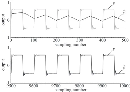
Fig. 2. Experimental results of system identification using quaternion neural network with 1–3–1 (H) network topology, where the grey line indicates plant output and the black line indicates output of the quaternion neural network (Top: initial adaptation stage of quaternion neural network; bottom: final adaptation stage of quaternion neural network).
norm
a
li
z
e
d c
os
t func
ti
on
CNN HNN BNN QNN
0.1
0.01
[image:3.595.312.538.53.214.2]0.001
Fig. 3. Comparison of normalized cost function obtained by the hypercomplex–valued neural network–based direct transfer function iden-tifiers (CNN: complex neural network with 2–5–1 (C) network topology; HNN: hyperbolic neural network with 2–5–1 (D) network topology; BNN: bicomplex neural network with 1–3–1 (T) network topology; QNN: quater-nion neural network with 1–3–1 (H) network topology).
neural network was defined as ξ(t) = y(t−1) +y(t −
2)i+u(t−1)j+u(t−2)k. The estimated plant output comprised one of the imaginary parts of the quaternion neural network’s output, that is, yˆ(t) = Imk[x(o)(t)], where Imk denotes the imaginary part of the imaginary unit k. Figure 2 shows an example of the system response when the direct transfer function identifier consisted of the quaternion neural network with a 1–3–1 network topology. As shown in Fig. 2, the identifier output converges with the plant output. Figure 3 shows the normalized cost function averaged within one period of the reference input. Here, the normalized cost function is averaged using 100 results of each neural network within the range [9000, 10000]. The topology of each neural network was defined so that the number of parameters, such as weights and thresholds, corresponded to the number in the quantum neural network. The normalized cost function of the quaternion neural network is smaller than that of the other neural network. These results indicate the feasibility of the proposed direct transfer function identifier using the hypercomplex–valued neural network.
M = 1 M = 2 M = 3 M = 4 M = 5
1 2 3 4 5
order of input -13000
-11000
-12000
A
[image:4.595.333.515.51.225.2]IC
Fig. 4. Experimental results of quaternion neural network for finding optimal network topology based on AIC, whereMindicates the number of neurons in the hidden layer.
0 0.006
0.002 0.004
norm
al
iz
ed c
os
t func
ti
on closed test
open test
RNN CNN HNN BNN QNN
8-2-4 8-4-4 4-2-2 4-2-2 2-1-1 2-1-1
Fig. 5. Comparison of estimation performance obtained by the hypercomplex–valued neural network–based direct transfer function iden-tifiers (RNN: real number neural network; CNN: complex neural network; HNN: hyperbolic neural network; BNN: bicomplex neural network; QNN: quaternion neural network).
Franc) as the target system. Here, the total number of data points was 3523 (4/Jan./2002 ∼ 5/Aug./2016). We split the data into two sets, namely, training set (4/Jan./2002 ∼ 2/Jun./2009) and test set (3/Jun./2009 ∼ 5/Aug./2016). The training set was used in closed tests for evaluating the training accuracy, while the test set was used in open tests for evaluating the estimation accuracy of the proposed direct transfer function identifiers. Assuming that the dynamics of historical data can be represented by the autoregressive
(AR) model yl(t) = m ∑
s=1
alsyl(t−s) +ul(t)(l= 1,2,3,4),
the input vector of the hypercomplex–valued neural network in the direct transfer function identifier was defined as ξ(t) = [ y(t−1) y(t−2) · · · y(t−m) u(t) ]T. In the experiments,y1,y2,y3andy4denoted the currency pairs USD/JPY, GBP/JPY, EUR/JPY and CHF/JPY, respectively, and ul(t) was random noise generated in the interval
[−0.02,0.02]. Figure 4 shows the result of network topology optimization of the quaternion neural network by using the Akaike Information Criterion (AIC) in the closed test. Here the components of the input vector were y=y1+y2i+y3j+y4kandu=u1+u2i+u3j+u4k, while the estimation results were given by yˆ(t) = [ Re[x(o)(t)] Imi[x(o)(t)] Imj[x(o)(t)] Imk[x(o)(t)] ]T.
1 2
3 4
5
Fig. 6. Representation of movement ‘Push down and stand on one leg’ in 24–formTaijiquanwith CG model based on captured motion data.
[image:4.595.56.283.54.232.2]As shown in Fig. 4, the optimal order of the input m is one and the optimal number of neurons in the hidden layer M is one because of the lowest number of the AIC. Figure 5 shows the normalized cost function averaged within the range of each test. Here, the normalized cost function is averaged using 20 results of each neural network. Although the normalized cost functions in the closed test are almost identical, the normalized cost function of each hypercomplex–valued neural network in the open test is smaller than that of the real number neural network. These results indicate the effectiveness of the hypercomplex–valued neural network in applications involving multiple–input multiple–output system identification.
Next, the direct transfer function identifier was applied to estimate human movements acquired by an optical motion capture system. Here, the basic routine of 24–formTaijiquan
was considered as the movement and the motion data of the movement ‘Push down and stand on one leg’, shown in Fig. 6, in which one arm is raised and the other is lowered while simultaneously standing on one leg – a crouching step changes the high position to a low one and then one leg is raised with a weight supported by the other one – was used as the target system. A subject (Japanese male, age: 22, height: 177 cm) who learned Taijiquan for six months from aTaijiquan instructor performed the movement twice, and the 3D motion data of 36 body parts were captured at a sampling rate of 30 fps [17]. In the motion capture system, the x– and the z–axes comprise the horizontal plane, and the y–axis is perpendicular to the aforementioned plane. In the computational experiment, 3D motion data of the head (xh(t), yh(t), zh(t)) and centre of the waist
(xw, yw(t), zw(t)) were considered as the target data. The
total number of data points was 2646, and the data was split up into two sets – training set covering the range [0, 1322] and test set covering the range [1323, 2646]. Given that the motion had a constant acceleration characteristic, the second–order AR model was assumed to define the input vector of the hypercomplex–valued neural network ξ(t) = [ yh(t−1) yw(t−1) yh(t−2) yw(t−2) uh(t)
uw(t) ]T, where yl = xli + ylj + zlk and
[image:4.595.55.284.291.414.2]0 1000 2000 3000 0
0.5
norm
al
iz
ed pos
iti
on
z
0.6 1.0
norm
al
iz
ed pos
iti
on
y
0 0.5
norm
al
iz
ed pos
iti
on
x
x x
^
y y
^
z z
^
closed test open test
closed test open test
closed test open test
sampling number
0 1000 2000 3000
0 0.5
norm
al
iz
ed pos
iti
on
z
0 0.5
norm
al
iz
ed pos
iti
on
y
0 0.5
norm
al
iz
ed pos
iti
on
x
x x
^
y y
^
z z
^
closed test open test
closed test open test
closed test open test
sampling number (a) head position
(b) waist position
h h
h h
h h
w w
w w
[image:5.595.56.287.55.519.2]w w
Fig. 7. Experimental results of motion data estimation using quaternion neural network with 6–2–2 (H) network topology; the black line indicates the measured data and the grey line indicates the output of the quaternion neural network (Top: 3D position of head, bottom: 3D position of waist).
head and waist were estimated from the imaginary parts of the quaternion neural network’s output:
ˆ
y(t) = [ Imi[x(o)(t)] Imj[x(o)(t)] Imk[x(o)(t)] ]T. Figure 7 shows the system response for the case in which the direct transfer function identifier consisted of a quaternion neural network with a 6–2–2 network topology. As shown in the figure, the output of the quaternion neural network could approximate the motion data in the closed and the open tests. This result indicates the usefulness of the proposed direct transfer function identifier using the hypercomplex–valued neural network.
IV. CONCLUSIONS
In this study, the capability of hypercomplex–valued neural networks was investigated and their application to system
identification was explored. A direct transfer function iden-tifier in which the output of a target system is estimated by the multilayer hypercomplex–valued neural network was de-signed and its characteristics were evaluated. Computational experiments using a complex neural network, hyperbolic neural network, bicomplex neural network and quaternion neural network were conducted to estimate the output of a discrete–time dynamic plant, historical foreign exchange data and the motion data ofTaijiquanmovements. The experimen-tal results confirmed the feasibility and effectiveness of the proposed hypercomplex–valued neural network–based direct transfer function identifier.
REFERENCES
[1] B. K. Tripathi, High Dimensional Neurocomputing - Growth, Ap-praisal and Applications -, Springer India, 2015.
[2] T. Nitta (ed.), Complex–Valued Neural Networks - Utilizing High– Dimensional Parameters -, Information Science Reference, 2009. [3] A. Hirose (ed.), Complex–Valued Neural Networks - Advances and
Applications -, IEEE Press, WILEY, 2013.
[4] L. Fortuna, G. Muscato and M. G. Xibilia, “A Comparison Between HMLP and HRBF for Attitude Control”,IEEE Transactions on Neural Networks, Vol. 12, No. 2, pp. 318–328, 2001.
[5] H. Kusamichi, T. Isokawa, N. Matsui, Y. Ogawa and K. Maeda, “A New Scheme Color Night Vision by Quaternion Neural Network”, in Proceedings of the 2nd International Conference on Autonomous Robots and Agents, pp. 101–106, 2004.
[6] P. Arena, R. Caponetto, L. Fortuna, G. Muscato and M. G. Xibilia, “Quaternionic Multilayer Perceptrons for Chaotic Time Series Predic-tion”, IEICE Transactions Fundamentals, Vol. E79–A, No. 10, pp. 1682–1688, 1996.
[7] S. Buchholz and N. Le Bihan, “Optimal Separation of Polarized Signals by Quaternionic Neural Networks”, in Proceedings of 14th European Signal Processing Conference, pp. 1–5, 2006.
[8] B. C. Ujang, C. C. Took and D. P. Mandic, “Quaternion–Valued Non-linear Adaptive Filtering”, IEEE Transactions on Neural Networks, Vol. 22, No. 8, pp. 1193–1206, 2011.
[9] F. Shang and A. Hirose, “Quaternion Neural–Network–Based PolSAR Land Classification in Poincare–Sphere–Space”,IEEE Transactions on Geoscience and Remote Sensing, Vol. 52, No. 9, pp. 5693–5703, 2014. [10] T. Ogawa, “Neural Network Inversion for Multilayer Quaternion Neural Networks”, Computer Technology and Applications, Vol. 7, pp. 73–82, 2016.
[11] Y. Cui, K. Takahashi and M. Hashimoto, “Design of Control Systems Using Quaternion Neural Network and Its Application to Inverse Kinematics of Robot Manipulator”, inProceedings of 2013 IEEE/SICE International Symposium on System Integration, pp.527–532, 2013. [12] K. Takahashi, Y. Hasegawa and M. Hashimoto, “Remarks on
Quater-nion Neural Network-based Self–tuning PID Controller”, in Proceed-ings of the 3rd International Symposium on Computer, Consumer and Control, pp.231–234, 2016.
[13] K. Takahashi, Y. Wakaume, T. Hirayama and M. Hashimoto, “Remarks on Hypercomplex–valued Neural Network–based Direct Adaptive Controller”, in Proceedings of the 2nd International Conference on Robotics and Automation Sciences / International Conference on Multimedia Systems and Signal Processing, S18, 2016.
[14] T. Isokawa, H. Nishimura and N. Matsui, “Quaternionic Multilayer Perceptron with Local Analyticity”,Information, Vol. 3. pp. 756–770, 2012.
[15] B. C. Ujang, C. C. Took and D. P. Mandic, “Split Quaternion Nonlinear Adaptive Filtering”,Neural Networks, Vol. 23, No. 3, pp. 426–434, 2010.
[16] E. Hitzer, “Algebraic Foundations of Split Hypercomplex Nonlinear Adaptive Filtering”,Mathematical Methods in the Applied Sciences, Vol. 36, No. 9, pp. 1042–1055, 2013.