Published Online October 2012 in SciRes (http://www.SciRP.org/journal/ojf) http://dx.doi.org/10.4236/ojf.2012.24027
Effect of Spatial Scale on Modeling and Predicting Mean Cavity
Tree Density: A Comparison of Modeling Methods
Stephen S. Lee
1, Zhaofei Fan
2*1Department of Statistics, College of Science, University of Idaho, Moscow, USA 2Forest and Wildlife Research Center, Mississippi State University, Starkville, USA
Email: [email protected], *[email protected]
Received June 5th, 2012; revised July 13th, 2012; accepted August 1st, 2012
Cavity trees are integral components of healthy forest ecosystems and provide habitat and shelter for a wide variety of wildlife species. Thus, monitoring and predicting cavity tree abundance is an important part of forest management and wildlife conservation. However, cavity trees are relatively rare and their abundance can vary dramatically among forest stands, even when the stands are similar in most other re-spects. This makes it difficult to model and predict cavity tree density. We utilized data from the Missouri Ozark Forest Ecosystem Project to show that it is virtually impossible to accurately predict cavity tree occurrence for individual trees or to predict mean cavity tree abundance for individual forest stands. However, we further show that it is possible to model and predict mean cavity tree density for larger spa-tial areas. We illustrate the prediction error monotonically decreases as the spaspa-tial scale of predictions in-creases. We successfully explored the utility of three classes of models for predicting cavity tree probabil-ity/density: logistic regression, neural network, and classification and regression tree (CART). The results provide valuable insights into methods for landscape-scale mapping of cavity trees for wildlife habitat management, and also on sample size determination for cavity tree surveys and monitoring.
Keywords: CART, Logistic Regression; Neural Network; Oak Forest; Prediction Accuracy
Introduction
Spatial prediction (mapping) of rare forest components such as cavity trees is an important topic in resource management and planning intended to conserve wildlife habitat. Cavity trees are live or dead trees with holes that occur naturally or that are excavated by certain wildlife species. In Missouri, more than 89 wildlife species require cavity trees or snags (Titus, 1983), and cavity tree availability is one of the most important factors for success of populations of cavity-nesting birds (McClelland & Frissell, 1975).
Extensive analyses regarding factors contributing to cavity tree formation and abundance prediction in oak forests have been reported previously (Fan et al., 2003a, 2003b, 2004a, 2004b, 2005). The biggest obstacle in cavity tree prediction for individual trees, for inventory plots (typically 0.1 to 0.2 ha in size), and for forest stands (typically 5 to 20 ha in size) results from the rareness of cavity trees and their large spatial and temporal variation. This large variation occurs because forma-tion of cavities is predominately the consequence of a set of random or semi-random events such as fire, insect attack, dis-ease, animal excavation, mechanical or chemical injury, and subsequent decay (Carey, 1983). However, at large spatial scales cavity tree probability and abundance can be predicted with reasonable accuracy using tree and stand attributes as in-dicators of the underlying cavity tree formation processes or causes (Fan et al., 2004a, 2005).
At the individual tree level, there are numerous statistical methods such as logistic regression, neural network, and classi-fication and regression tree (CART) analysis that can be used to
predict the probability that a given tree is a cavity tree and/or to identify contributing factors associated with cavity abundance. CART has been shown to be especially promising for estimat-ing cavity tree abundance at multiple spatial scales (Fan et al., 2004b, 2005). For cavity tree estimation, CART can explicitly identify significant contributing tree and/or plot (stand) factors (and their critical threshold values) and potential interactions in a hierarchical (nested) structure. CART identifies categories of observations (nodes) that maximize the separation of cavity trees from trees without cavities. Nodes quantify cavity tree probabilities, but they also identify discrete categories that can be used with aggregation or resampling methods to predict cavity tree abundance at any spatial scales greater than individ-ual trees (e.g., plots, stands, small or large landscapes) (Fan et al., 2004a).
re-sampled versions of the original data set will result in models that are substantially different.
The objective of this study was to compare the predic-tion/classification accuracy of binary cavity tree data using CART and two other commonly used statistical methods: neu-ral network and logistic regression. We compared the single “best” model from each method with one another as well as with 50 Bagged models for neural network and CART. The logistic regression model is relatively stable with respect to data bootstrapping, so we did not use it to build Bagged models. However, we still investigated the prediction accuracy of its single “best” model because it is one of the most commonly used generalized linear models for binary data. From a model- selection perspective, we quantitatively evaluated the effec-tiveness of aggregating the single “best” CART model and the 50 Bagged CART models at multiple spatial scales. The infor-mation is specifically useful in mapping and monitoring the cavity tree resource for wildlife. More generally the findings demonstrate how rare, natural phenomena can be quantified and predicted by a variety of single and bagged modeling tech-niques.
Methods
Study Site and Data
The Missouri Ozark Highlands are dominated by second- growth oak-hickory and oak-pine forests which originated when native forests were heavily harvested in the early 1900s. Since then, most forests have experienced periodic partial har-vesting and frequent low-intensity fires. White oak (Quercus
alba L.), black oak (Quercus velutina Lam.), scarlet oak
(Quercus coccinea Muenchh.), post oak (Quercus stellata
Wangenh.), shortleaf pine (Pinus echnina Mill.), blackgum
(Nyssa sylvatica Marsh.), and hickory (Carya) species account
for over 94 percent of trees in the forest canopy in terms of importance value. For management purposes, forests are or-ganized into “stands” which are reasonably homogenous, con-tiguous groups of trees that are typically 2 to 20 ha in extent. The majority of forest stands in the study area are dominated by trees at least 60 years old. The Missouri Ozark Forest Ecosys-tem Project (MOFEP), initiated by the Missouri Department of Conservation in 1989, is a century-long, landscape-scale ex-periment to examine the effects of alternative forest manage-ment practices on multiple ecosystem attributes. MOFEP uses a randomized complete block design with nine sites (experimen-tal units with multiple stands) that range from 314 to 516 ha in size and are organized into three blocks (Sheriff & He, 1997, Sheriff 2002). The MOFEP woody vegetation inventory sur-veyed more than 50,000 individual trees >11 cm dbh and their associated environmental factors including slope, aspect, geo- landform, soil, and ecological land type (ELT). The measured trees were on 648 permanent 0.2-ha circular plots across the nine experimental sites and were measured both before and after treatment alternatives were applied (Brookshire & Shifley, 1997; Sheriff & He, 1997). The tree species, diameter at breast- height (dbh), crown class, decay class (for dead trees, called snags), and cavity presence/absence were recorded for each tree. For this study, a cavity was defined as a hole with a diameter no less than 2.5 cm that appeared dark inside (Jensen et al., 2002). Based on prior findings of Fan et al. (2003a), we used the fol-lowing four covariates to predict cavity tree probability: species group (ten groups), decay class (from I to VII indicating
in-creasing level of decomposition), diameter at breast height (dbh, measured in cm at a height of 1.4 m above ground level), and tree status (live or dead).
Statistical Modeling
Predicting Cavity Tree Probability at Individual Tree-Level
Given a training data set T ={(xi, yi), i = 1,, n = n0 + n1} =
{(xi, 0), i = 1,, n0} {(xi, 1), i = 1,, n1}, we would like to
develop the assignment rules for future unknown objects using the explanatory vector x. In the case of binary classification, they could be viewed as methods to estimate the condition probability,
1|
1
0 |
f x P y x P y x
(1)
where x is any point in the 4-dimensional state space of the four
covariates mentioned above. In this study, we used three types of classification models: neural networks, logistic regression, and classification and regression tree (CART) to predict cavity tree probability at the individual-tree level. The three models applied in the study are outlined in the following sections. De-tailed descriptions of the general modeling techniques can be found in many textbooks (e.g., Ripley, 1996).
Neural Networks (NN)
There are many kinds of neural networks (see Hertz et al., 1991 for an introduction), but in this paper we restrict ourselves to only supervised, feedforward, single-hidden-layer neural networks with a logistic output activation function. The esti-mate of f x
is
0 0 41
ˆ ˆ ˆ ˆ ˆ
h h jh j
h j
f x w w w w x
(2)
where w w wˆ ˆ ˆ0, h, 0h,wˆjh are the connection weights and
1
. This type of network has 4 units at the1 exp
input layer, h hidden units at the middle hidden layer, and 1
output unit at the output layer. Such networks are very general and we denote them by the notation 4-h-1 NN. It has been
shown by many authors that, for sufficiently large h, any con-tinuous real-valued function f x
in the 4-dimensional spacecan be approximated by these 4-h-1 NN to any desirable degree
of accuracy. The number of hidden units h is found by cross
validation to prevent model overfitting.
Logistic Regression (LG)
The model is
40 1
log j j
j
it f x x
(3)
where log
log 1z it z
z
,
and
β’s
are the parameters to be estimated via maximum like-lihood (Myers, 1990).Classification and Regression Tree (CART)
mogeneous regions, often hypercubes parallel to the variable axes. There are many different schemes for estimating classifi-cation trees. The basic idea is to recursively choose a variable or combination of variables and to split the variable’s space on a carefully chosen value. These schemes differ in allowing multi-way splits or restricting binary splits and in deciding how the best split is completed. Also, they differ in when to stop growing the tree and how to prune it back for generalization. The conditional probability ˆ( )f x is estimated to be the
pro-portion of y = 1 observations among those in the terminal node
containing the prediction point x. We used the Splus tree
classi-fier which is based on the well-known Breiman’s CART (Bre-iman et al., 1984). For a given training data set, we fit two kinds of trees: a full-grown tree with no pruning and a pruned classification tree obtained from the full-grown tree by snipping off the least important splits according to a cost-complexity factor (Venables & Ripley, 1994).
Prediction Assessment for Individual Cavity Trees
We measured the 10-fold cross validation error rate to assess both the single “best” model and the 50 Bagged models using the following five commonly accepted statistical criteria: Re-ceiver Operating Characteristic (ROC) area, Misclassification Rate (MR), Mean Absolute Deviation (MAD), Root Mean Square Error (RMSE), and Kullback-Leibler (KL) Distance. The first two are measures of discrimination and the last three are measures of calibration. MR, MAD, and RMSE are widely used in regression analyses and readily interpretable in most applied research. We describe ROC area and KL distance be-low.
ROC Area
In the binary case, let class 0 be termed negative outcomes and class 1 as positive outcomes. A new case is classified as positive if f xˆ
is larger than or equal to a pre-chosenthreshold value; otherwise, the case is classified as negative. An ROC curve is a plot of the true positive rate versus the false positive rate of a classification rule as the threshold value varies from 0 to 1. The true positive rate is defined as the number of positives correctly classified, divided by the total number of positives; the false positive rate is defined as the number of negatives incorrectly classified, divided by the total number of negatives. An ideal model would have an ROC area equal to 1.0 (completely separable) since the true positive rate is 1 and the false positive rate is 0 regardless of the threshold value. By comparing ROC areas, dominance relationships between classi-fiers can be defined. The dominance relationship is clear when the ROC curve from one model is always above the curve of another, and the two curves do not intersect. When they do intersect, one model is superior in some regions and another elsewhere. The area under the curve becomes an average col-lective overall comparison between models. Accordingly, a model with a larger ROC area is better than a model with smaller ROC area.
KL Distance
KL distance measures the closeness between the observed yi given xi andthe predicted
f x
ˆ
i for all i, via
1
log ˆ 1 log ˆ
1 i
i i
i i
y y
y y
f x f x
i
i
(4)
The smallest distance is obviously 0 which happens when f xˆ
i yi,i. Discrimination and calibration are tworelated yet different measures. Although a model with good discrimination tends to have good calibration and vice versa, a model may appear to be strong in one measure but weak in the other. Harrell et al. (1996) recommended that good discrimina-tion be preferred to good calibradiscrimina-tion since a model with good separability can always be recalibrated, but the rank orderings of probabilities cannot be changed to improve separation. Therefore, we used ROC as the guiding measure for model assessment.
Predicting Cavity Tree Density (CTD) at Different
Spatial Scales over Plot Size
Spatial scale is a crucial factor in the prediction accuracy of CTD (Fan et al., 2005). In general, the prediction accuracy of mean cavity tree density increases with increasing area (e.g., increasing plot size or stand area), but managers faced with conservation decisions desire methods that provide a good bal-ance between spatial resolution (finer is preferable) and predic-tion accuracy (higher is preferable). To compare how the en-semble of Bagged CART models differ from the single “best” CART model in predicting CTD at different spatial scales, we split the 648 plots into two groups: a construction set and a validation set, respectively. We used the construction set to build the single “best” CART model and a set of 50 Bagged CART models. Given cavity tree probability (pi) for the total
number (ni) of trees (cavity trees and non-cavity trees) classi-fied into terminal node i of the CART model specified by tree species, dbh, decay class and their threshold values, then the single “best” CART estimate of CTD for a forest area of size A (ha) can be predicted as the mean of all s terminal nodes as follows,
1ˆ CTD #/ ha
A s
i i i
p n
(5)
with respect to the 50 Bagged CART models, CTD for the en-semble of 50 models can be predicted as,
50
1 1
ˆ CTD #/ ha
50A
i s
ij ij i j
p n
(6)
where si is the number of terminal nodes for model i.
We randomly merged the plots in the validation group to represent forest areas of increasing size, A, by groups of multi-ple plots. We calculated the observed and the predicted CTD, respectively, corresponding to each size of A. We ran the merging process 100 times for the validation group by picking different starting plots and merging the remaining plots in a different order. We plotted relative error (predicted-observed)/ observed) against spatial scale, A, to visualize the effect of spatial scale on prediction accuracy, via the single “best” model and the ensemble of 50 Bagged models.
Results
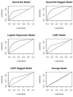
CART. Results for RMSE, MAD and MR did not differ greatly among the methods. Bagging improved prediction accuracy for neural network models, but the improvement was marginal for the CART model (Table 1 and Figure 1). The single “best” models and the ensembles of bagged models for each estima-tion technique were more accurate than a mean (average) ref-erence model determined by randomly assigning trees to classes. This indicates that chosen covariates (predictors) were, in fact, associated with cavity formation processes or causes and ap-propriate for this study.
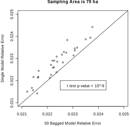
models always outperformed the single “best” model at spa-tial scales ranging from 1 to 70 ha, and particularly at small spatial scales (e.g., <10 ha). Although CART was not particu-larly useful at the individual tree level to predict single cavity trees, the bagged CART ensemble was the best model to predict CTD on the landscape level. The difference in relative error between the single and bagged CART models remains statisti-cally significant at 70 ha, the largest scale we examined, even though differences tend to decrease as the spatial scale in-creases (Figures 2-4).
Discussion
The scarcity of cavity trees and their great spatial and tem-poral variation present real challenges to managers interested in monitoring the cavity tree resource and to those who attempt to create models or tools to assist managers (Fan et al., 2003b; Eskelson et al., 2009). Cavity trees are difficult to be accurately observed from the ground (Jensen et al., 2002) and costly to inventory. Techniques to predict the dynamics and distribution of cavity trees as a function of known tree or forest characteris-tics and environmental gradients are needed to improve the efficiency of conservation practices. There are practical limits to the spatial resolution of cavity tree models that can be ap-plied to hardwood forests, even when models are based on ceptional data sets such as those created by the MOFEP ex-periment.
Table 1.
Comparison of modeling methods for cavity tree probability. Models (rows) are neural network (NN), 50 Bagged neural network (NN.bagg), logistic (LG), classification and regression tree (CART), 50 Bagged CART (CART.bagg), and mean model (Average). Evaluation statistics (columns) are receiver operating characteristic (ROC area), misclassi-fication rate (MR), mean absolute deviation (MAD), root mean square error (RMSE), and KL distance. The “Average” model uses the average
y value to predict future new cases, i.e., it ignores the 4 covariates in the
model building process.
Model ROC area MR MAD RMSE distanceKL
NN 0.730 0.0355 0.0532 0.174 1.759
NN.bagg 0.856 0.0356 0.0511 0.172 0.118
LG 0.859 0.0355 0.0580 0.172 0.117
CART 0.713 0.0356 0.0618 0.176 0.132
CART.bagg 0.733 0.0356 0.0621 0.175 0.130 Average* 0.485 0.0356 0.0686 0.185 0.154
We found logistic regression was most accurate with an ROC In this study we explored three commonly used classification models for binary data: neural network, logistic regression and CART and evaluated their prediction accuracy by five criteria. area of 0.859, CART was the least accurate with an ROC area of 0.713, and neural network was intermediate with an ROC area of 0.730. But none of the methods were able to account for the majority of variation of cavity tree occurrence and distribu-tion at the individual-tree level.
Small-scale statistical modeling approaches (e.g., based on individual tree, plot, or stand scales) are overwhelmed by the variation inherent in the cavity tree resource. Understanding the magnitude of this variability is essential to understanding cavity tree resource dynamics. It is virtually impossible to accurately predict whether or not an individual tree will be a cavity a tree or to accurately predict the number of cavity trees per acre for a given inventory plot or stand (Fan et al., 2003b). However, at large spatial scales (e.g. >30 ha), it is possible to derive esti-mates of mean cavity tree abundance that are useful to manag-ers (Fan et al. 2004b). Based on our findings for CART models (Figures 2 and 3), relative error of cavity tree estimates
de-creases sharply as the minimum area used in estimation in-creases to 30 ha (i.e., as the model resolution dein-creases), and relative error continues to decrease as the minimum area in-creases to 70 ha (the largest area and coarsest resolution we examined), which agrees with Fan et al. (2004a).
Bagging to derive ensembles of equally likely models that “vote” on an outcome can improve the performance of neural network and CART models, but the ROC area of bagged neural network and CART models was still less than logistic regres-sion (Table 1, Figure 1). Based on the other four criteria, the
bagged and the single “best” models were nearly identical. It is important to develop appropriate statistical models that accurately quantify cavity tree distribution at sampling scales useful for managers (e.g., Lawler & Edwards, 2002). Consider-ing the simplicity (summation as illustrated by Equations (5) and (6)) and applicability (trees are grouped into one of the limited number of groups explicitly specified by tree attributes) of three models in aggregation over scales, we found the CART to be especially amenable to predictions of CTD across a range of different spatial scales.
The relative prediction errors exponentially decrease as spa-tial scale increases for both the single “best” model and ensem-bles of 50 bagged CART models (Figures 2 and 3). The
asso-ciation between relative error and spatial scale provides essen-tial information for applying cavity tree models and interpreting results. Figures 2 and 3 describe the relationship between
0.0 0.2 0.4 0.6 0.8 1.0
0.
0
0
.4
0.
8
1-specificity
s
e
ns
it
iv
it
y
Neural Net Model
0.0 0.2 0.4 0.6 0.8 1.0
0.
0
0
.4
0.
8
1-specificity
s
e
ns
it
iv
it
y
Neural Net Bagged Model
0.0 0.2 0.4 0.6 0.8 1.0
0.
0
0.
4
0
.8
1-specificity
s
e
n
s
it
iv
it
y
Logistic Regression Model
0.0 0.2 0.4 0.6 0.8 1.0
0.
0
0.
4
0
.8
1-specificity
s
e
n
s
it
iv
it
y
CART Model
0.0 0.2 0.4 0.6 0.8 1.0
0.
0
0.
4
0.
8
1-specificity
s
ens
it
iv
it
y
CART Bagged Model
0.0 0.2 0.4 0.6 0.8 1.0
0.
0
0.
4
0.
8
1-specificity
s
ens
it
iv
it
y
[image:5.595.144.438.82.474.2]Average Model
Figure 1.
Receiver operating characteristic (ROC) area of logistic regression, neural network and CART in cavity tree probability prediction.
20 30 40 50 60 70
0.
02
0.
03
0
.04
0.
05
0.
06
0.
07
Relative error versus sampling area: 20 to 70 ha
Sampling area in ha
R
e
la
ti
v
e
e
rro
r
0.
02
0.
03
0
.04
0.
05
0.
06
0.
07
1 3 5 7 9 11 13 15 17 19
0
.0
5
0
.10
0
.15
0.
20
0.
25
0.
30
0.
35
0.
4
0
Relative error versus sampling area: 1 to 20 ha
Sampling area in ha
R
e
la
ti
v
e
e
rr
o
r
0
.0
5
0
.10
0
.15
0.
20
0.
25
0.
30
0.
35
0.
4
0
[image:5.595.70.276.519.703.2]Single Model 50 Bagged Model
Figure 2.
Change of relative errors with spatial scale (from 1 to 20 ha) for single and Bagged CART models for predicting cavity tree density.
Figure 3.
[image:5.595.324.521.523.703.2]0.021 0.022 0.023 0.024 0.025
0.
021
0.
02
2
0
.0
23
0.
02
4
0
.0
25
Sampling Area is 70 ha
50 Bagged Model Relative Error
Si
ng
le
M
o
de
l
Rel
at
iv
e
E
rr
o
r
[image:6.595.68.279.87.293.2]t test p-value < 10^-9
Figure 4.
Scatter plot of relative errors of single and 50 Bagged models at a spatial scale of 70 ha.
Conclusion
This study constructs three classes of tree-level models to es-timate probabilities of cavity presence: logistic regression, neu-ral networks, and CART. The estimated probabilities are com-bined with known tree counts within covariate classes to predict mean cavity tree density at different spatial scales, with or without bootstrap aggregation (bagging). Although logistic regression was the best model to predict cavity probabilities at the individual tree level, the bagged CART outperformed other models in predicting mean cavity tree density at the landscape scale (e.g., >10 ha). Prediction accuracy, measured in terms of relative error continues to decrease with spatial scale and the difference between the bagged CART ensemble and single CART model remains significant statistically at largest spatial scale (70 ha) tested in the study. This is largely due to the non-stationary nature of CART. In addition, the tree profile and explicit deposition of important covariates in a one-after-an- other manner of CART make it more useful for landscape level cavity tree mapping.
Acknowledgements
Mr. Randy Jensen from Missouri Department of Conserva-tion provided cavity tree data used for these analyses. Dr. Stephen R. Shifley from USDA Forest Service Northern Re-search Station reviewed the first draft of this paper. Dr. Michael K. Crosby from the Department of Forestry, Mississippi State University helped formatting and reviewing the revised version of this paper. We thank them all.
REFERENCES
Breiman, L. (1995). Stacked regressions. Machine Learning, 24, 49-64.
doi:10.1007/BF00117832
Breiman, L. (1996). Bagging predictors. Machine Learning, 26, 123- 140. doi:10.1007/BF00058655
Breiman, L., Friedman, J. H., Olshen, R. A., & Stone, C. J. (1984).
Classification and regression trees. Monterey, CA: Wadsworth and
Brooks.
Brookshire, B. L., & Shifley, S. R. (Eds.) (1997). Proceedings of the missouri ozark forest ecosystem project symposium: An experimental approach to landscape research, St. Louis, 3-5 June 1997.
Carey, A. B. (1983). Cavities in trees in hardwood forests. Snag habitat management symposium. General Technical Report GTR-RM-99, US Department of Agriculture Forest Service, 167-184.
Eskelson, B. N., Temesgen, H., & Barrett, T. M. (2009). Estimating ca- vity tree and snag abundance using negative binomial regression models and nearest neighbor imputation methods. Canadian Journal of Forest Research, 39, 1749-1765. doi:10.1139/X09-086
Fan, Z., Larsen, D. R., Shifley, S. R., & Thompson III, F. R. (2003a). Estimating cavity tree abundance by stand age and basal area, Mis-souri, USA. Forest Ecology and Management,179, 231-242.
doi:10.1016/S0378-1127(02)00522-4
Fan, Z., Lee, S., Shifley, S. R., Thompson III, F. R., & Larsen, D. R. (2004a). Simulating the effect of landscape size and age structure on cavity tree density using resampling technique. Forest Science,50,
603-609.
Fan, Z., Shifley, S. R., Spetich, M. A., Thompson III, F. R., & Larsen, D. R. (2003b). Distribution of cavity trees in Midwestern old-growth and second-growth forests. Canadian Journal of Forest Research,33,
1481-1494. doi:10.1139/x03-068
Fan, Z., Shifley, S. R., Spetich, M. A., Thompson III, F. R., & Larsen, D. R. (2005). Abundance and size distribution of cavity trees in sec-ond-growth and old-growth central hardwood forests. Northern Journal of Applied Forestry,22,162-169.
Fan, Z., Shifley, S. R., Thompson III, F. R., & Larsen, D. R. (2004b). Simulated cavity tree dynamics under alternative timber harvest re-gimes. Forest Ecology and Management, 193, 399-412.
doi:10.1016/j.foreco.2004.02.008
Hand, D. J. (1997). Construction and assessment of classification rules.
New York, NY: Wiley.
Harrell Jr., F. E., Lee, K. L., & Mark, D. B. (1996). Multivariable prog-nostic models: Issue in developing models, evaluating assumptions and adequacy, and measuring and reducing errors. Statistics in Medi-cine,15, 361-387.
doi:10.1002/(SICI)1097-0258(19960229)15:4<361::AID-SIM168>3. 0.CO;2-4
Hertz, J. A., Krogh, A. S., & Palmer, R. G. (1991). Introduction to the theory of neural computation. Redwood City, CA: Addison-Wesley. Jensen, R. G., Kabrick J. M., & Zenner, E. K. (2002). Tree cavity
esti-mation and verification in the Missouri Ozarks. General Technical Report GTR-NC-1227, US Department of Agriculture Forest Service, 114-129.
Johnson, R. A., & Wichern, D. W. (1992). Applied Multivariate Statis-tical Analysis. Upper Saddle River, NJ: Prentice Hall.
Lawler, J. J., & Edwards, T. C. (2002). Landscape patterns as predictors of nesting habitat: Building and testing models for four species of cavity-nesting birds in the Uinta Mountains of Utah, USA. Land-scape Ecology,17, 233-245. doi:10.1023/A:1020219914926 McClelland, B. R., & Frissell, S. S. (1975). Identifying forest snags
useful for hole-nesting birds. Journal of Forestry,73, 414-417. Myers, R. H. (1990). Classical and Modern Regression with
Applica-tions. Boston: PWS Publishing Company.
Ripley, B. D. (1996). Pattern recognition and neural networks. Cam-bridge: Cambridge University Press.
Sheriff, S. L. (2002). Missouri ozark forest ecosystem project: The ex- periment. General Technical Report GTR-NC-227, US Department of Agriculture Forest Service, 1-25.
Sheriff, S. L., & He, Z. (1997). The experimental design of the Missouri Ozark Forest Ecosystem Project. General Technical Report GTR-
NC-193, US Department of Agriculture Forest Service, 26-40. Titus, R. (1983). Management of snags and cavity trees in Missouri—A
process. Snag habitat management symposium. General Technical
Report GTR-RM-99, US Department of Agriculture Forest Service, 51-59.
Venables, W. N., & Ripley B. D. (1994). Modern applied statistics with S-plus. New York: Springer-Verlag.
Wolpert, D. (1992). Stacked generalization. Neural Networks,5, 241-