Ancient dreams : a spectroscopic study of variable stars in binary systems

Department of Physics and Astronomy

A thesis submitted as part of the requirements

for the degree of Master of Science in Astronomy

Ancient Dreams: A spectroscopic

study of variable stars in binary

systems

Author:

Sanjay Sekaran

Senior Supervisor:

Assoc. Prof. Karen Pollard

Associate Supervisor:

Professor Mike Reid

“You must have chaos in your soul to give birth to a

dancing star.”

Abstract

This thesis presents the results of the orbital and asteroseismological analysis of three vari-able stars in binary systems:HD 182640, a system with a candidateγDoradus primary;HD 3112, a system with a bona fideδScuti primary; andHD 147787, a system with a candidate

γ Doradus primary. Approximately 2500 spectra of all three stars were obtained from the

HERCULESspectrograph, attached to the 1-metre telescope at the University of Canterbury

Mount John Observatory. The raw spectra were reduced to radial velocity line profiles through cross-correlation with synthetic spectra.

Orbital analysis ofHD 182640characterised it as a long period (1256 d) binary with an

eccentric orbit (e₌0.43). A total of 18 pulsational frequencies, explaining 42.9% of the varia-tion across the line profiles, were identified. These frequencies were all characterised as high-degree (` >4) modes.

Orbital analysis ofHD 3112characterised it as a short period (7 d) binary with an

effectively-circular orbit (e ₌0.01). A total of 17 pulsational frequencies, explaining 46.3% of the varia-tion across the line profiles, were identified. The mode of the primary pulsavaria-tion frequency (f₁₌20.2802 d−1_{) was the only one that was able to be identified. Previously identified}

ellip-soidal variations may have hindered mode identification efforts.

Orbital analysis ofHD 147787characterised it as a moderate period (40 d) binary with an

Declaration

I declare that all of the work presented in this Master’s thesis is my own, unless otherwise stated.

I would like to acknowledge the contributions of Dr. Duncan Wright, Dr. Emily Brunsden, Dr. Jovan Skuljian and Mr. Aaron Greenwood in writing and enhancing theMATLABscripts

used in the data reduction process. I would also like to acknowledge Dr. Christoph Bergmann for his help in creating the binary analysis methodology and for providing the radial velocity and orbital fitting codes. All other scientific software used in this analysis has been acknowl-edged and cited in the appropriate sections of this thesis.

I would also like to express my heartfelt gratitude to my senior supervisor, Associate Pro-fessor Karen Pollard, for all of her guidance and advice, and for proofreading this thesis.

Sanjay Sekaran

To Amma and Appa,

Contents

List of Figures _iv

List of Tables _viii

Glossary _xi

1 Introduction ₁

1.1 Ancient Dreams of the Universe . . . 1

1.2 Asteroseismology . . . 1

1.3 Stellar Pulsations . . . 3

1.3.1 Driving Mechanisms . . . 3

1.3.2 Radial Pulsations . . . 5

1.3.3 Non-Radial Pulsations . . . 5

1.3.4 Selection Mechanisms of Pulsation Modes and Frequencies . . . 7

1.3.5 Non-Radial Pulsational Geometry . . . 7

1.3.6 Rotational Effects on Pulsations . . . 9

1.3.7 Pulsational Effects on Spectroscopic Data . . . 12

1.4 Variable Star Classes . . . 13

1.4.1 γDoradus Variable Stars . . . 13

1.4.2 δScuti Variable Stars . . . 17

1.5 Binary Stars . . . 19

1.5.1 Binary Orbits . . . 20

1.5.2 Spectroscopic Binaries . . . 23

1.6 Thesis format and goals . . . 26

2 Data Collection and Analysis ₂₇ 2.1 Observational Data . . . 27

2.1.1 University of Canterbury Mount John Observatory (UC MJO) . . . 27

2.1.2 Observational Timeframe and Target Selection . . . 28

2.1.3 Observational Methodology . . . 29

2.2 Spectroscopic Data Reduction . . . 30

CONTENTS

2.2.2 First Data Reduction Pipeline . . . 30

2.2.3 Second Data Reduction Pipeline . . . 32

2.3 Binary Analysis . . . 36

2.3.1 Orbital Analysis . . . 37

2.3.2 Line Profile Correction . . . 40

2.4 Spectroscopic Variability Analysis . . . 41

2.4.1 Frequency Identification . . . 41

2.4.2 Mode Identification . . . 51

3 HD 182640 ₅₇ 3.1 Observations . . . 59

3.2 Binary Analysis . . . 59

3.3 Orbital Analysis . . . 62

3.4 Frequency Identification . . . 63

3.5 Mode Identification . . . 68

3.6 Discussion . . . 75

4 HD 3112 ₇₇ 4.1 Observations . . . 80

4.2 Orbital Analysis . . . 81

4.3 Frequency Identification . . . 83

4.3.1 The 13 d−1_{to 25 d}−1_{Frequency Range . . . . 83}

4.3.2 The 0 d−1_{to 3 d}−1_{Frequency Range . . . . 85}

4.3.3 Final Frequency Identification . . . 88

4.4 Mode Identification . . . 90

4.5 Discussion . . . 97

5 HD 147787 ₁₀₁ 5.1 Observations . . . 103

5.2 Orbital Analysis . . . 104

5.3 Frequency Identification . . . 105

5.4 Mode Identification . . . 110

5.5 Discussion . . . 114

6 Conclusion and Future Research ₁₁₇ 6.1 Conclusion . . . 117

6.2 Future Research . . . 119

CONTENTS

A Raw FITS Spectrum Examples ₁₂₃

B Additional Plots and Tables for HD 182640 ₁₂₇

C Additional Plots and Tables for HD 3112 ₁₃₉

D Additional Plots and Tables for HD 147787 ₁₅₉

List of Figures

1.1 Classes of variable stars on a Hertzsprung-Russell diagram. . . 4

1.2 Propagation ofp-mode andg-mode waves within a sun-like star. . . 6

1.3 Radial and Non-radial Pulsation Modes. . . 10

1.4 `₌20 Pulsation Modes. . . 11

1.5 Line Profile Variations due to Pulsations. . . 14

1.6 TheoreticalγDoradus instability strips for stars pulsating with`₌1 modes. . . . 16

1.7 TheoreticalδScuti instability strips for stars pulsating with`₌2 modes. . . 16

1.8 Schematic diagram of an elliptical orbit. . . 21

1.9 Eccentric and true anomalies on a diagram of a two-dimensional elliptical orbit. 22 1.10 Radial velocity curves of orbits with differente andω. . . 24

1.11 Doppler Shift of Spectral Lines in an SB2 Spectrum. . . 25

2.1 Barycentric correction values forHD 182640,HD 3112andHD 147787. . . 32

2.2 The continuum-fitting process for spectral order 99 ofHD 3112. . . 34

2.3 The mean stellar spectrum ofHD 182640. . . 35

2.4 The mean stellar spectrum of HD 147787with its correspondingδ-function template. . . 35

2.5 The cross-correlated line profiles ofHD 147787. . . 37

2.6 The Gaussian-fitting process forHD 3112. . . 38

2.7 The component orbital fits to the radial velocities ofHD 147787. . . 39

2.8 The line profilesHD 147787 A. . . 41

2.9 The iterative prewhitening process inFAMIASusing the pixel-by-pixel method. 45 2.10 The iterative prewhitening process inFAMIASusing the second moment of the moment method. . . 46

2.11 The spectral significance values of the frequencies of HD 3112identified by SigSpec. . . 48

2.12 The amplitude and phase profiles of f1=20.2802 d−1ofHD 3112. . . 50

2.13 The zero-point fit ofHD 182640. . . 54

LIST OF FIGURES

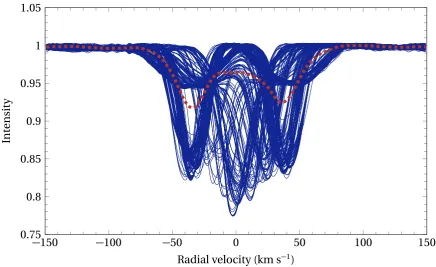
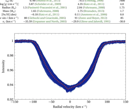
3.1 The cross-correlated line profiles ofHD 182640. . . 58

3.2 The partial Gaussian-fitting processes ofHD 182640 B. . . 60

3.3 The Gaussian-fitting process ofHD 182640 A. . . 60

3.4 The cross-correlated line profiles ofHD 182640 A. . . 62

3.5 The component orbital fits to the radial velocities ofHD 182640. . . 63

3.6 The 0 d−1 _{to 80 d}−1 _{frequency range pixel-by-pixel mean Lomb-Scargle} peri-odogram ofHD 182640. . . 64

3.7 The 0 d−1_{to 10 d}−1_{frequency range spectral window ofHD 182640. . . . 64}

3.8 The spectral significance values of the frequencies ofHD 182640identified by SigSpec. . . 65

3.9 Zero-point fit ofHD 182640. . . 69

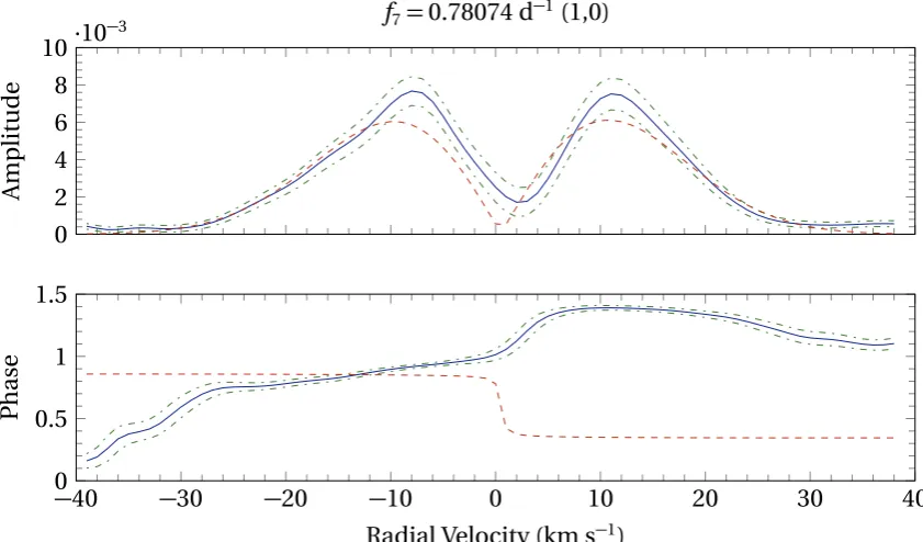
3.10 The amplitude and phase profiles of the best-fit modes off₁tof₆ofHD 182640. 72 3.11 The amplitude and phase profiles of the best-fit modes off₇tof₁₂ofHD 182640. 73 3.12 The amplitude and phase profiles of the best-fit modes off13tof18ofHD 182640. 74 4.1 The cross-correlated line profiles ofHD 3112. . . 79

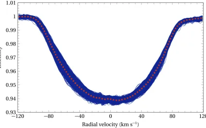
4.2 The cross-correlated line profiles ofHD 3112 A. . . 80

4.3 The component orbital fits to the radial velocities ofHD 3112. . . 82

4.4 The 0 to 80 d−1_{frequency range pixel-by-pixel mean Lomb-Scargle periodogram} ofHD 3112. . . 83

4.5 The spectral significance values of the frequencies ofHD 3112 identified by SigSpec. . . 84

4.6 The 13 to 25 d−1_{frequency range spectral window ofHD 3112. . . . 84}

4.7 The 0 d−1_{to 3 d}−1_{frequency range spectral window ofHD 3112. . . . 85}

4.8 Zero-point fit ofHD 3112. . . 91

4.9 Thev sini values of the models fit to the zero-point line profile ofHD 3112. . . . 92

4.10 The amplitude and phase profiles of the best-fit mode (1,1) off1=20.28 d−1of HD 3112. . . 93

4.11 The amplitude and phase profilesf₁tof₆ofHD 3112. . . 94

4.12 The amplitude and phase profiles off₇tof₁₂ofHD 3112. . . 95

4.13 The amplitude and phase profiles off₁₃tof₁₇ofHD 3112. . . 96

5.1 The cross-correlated line profiles ofHD 3112. . . .102

5.2 The cross-correlated line profiles ofHD 147787 A. . . .103

5.3 The component orbital fits to the radial velocities ofHD 147787. . . .105

LIST OF FIGURES

5.5 The spectral significance values of the frequencies ofHD 147787identified by

SigSpec. . . 106

5.6 The 0 to 6 d−1_{frequency range spectral window ofHD 147787. . . . 107}

5.7 Zero-point fit ofHD 147787. . . 111

5.8 Thev sini values of the models fit to the zero-point line profile ofHD 147787. . 112

5.9 The amplitude and phase profiles the best-fit modes of f1to f3, and f4to f7of HD 147787. . . 113

A.1 Flat-field spectrum example. . . 124

A.2 Thorium-Argon spectrum example. . . 125

A.3 Stellar spectrum example. . . 126

B.1 The first batch of five pixel-by-pixel mean Lomb-Scargle periodograms ofHD 182640. . . 128

B.2 The second batch of five pixel-by-pixel mean Lomb-Scargle periodograms of HD 182640. . . 129

B.3 The third batch of five pixel-by-pixel mean Lomb-Scargle periodograms ofHD 182640. . . 130

B.4 The fourth batch of three pixel-by-pixel mean Lomb-Scargle periodograms of HD 182640. . . 131

B.5 The zeroth-moment Lomb-Scargle periodograms ofHD 182640. . . 132

B.6 The first-moment Lomb-Scargle periodograms ofHD 182640. . . 133

B.7 The second-moment Lomb-Scargle periodograms ofHD 182640. . . 134

B.8 The third-moment Lomb-Scargle periodograms ofHD 182640. . . 135

B.9 Reduction in the standard deviation across the line profiles ofHD 182640. . . . 137

C.1 The first batch of five pixel-by-pixel mean Lomb-Scargle periodograms ofHD 3112(13 d−1to 25 d−1). . . 140

C.2 The second batch of five pixel-by-pixel mean Lomb-Scargle periodograms of HD 3112(13 d−1to 25 d−1). . . 141

C.3 The third batch of four pixel-by-pixel mean Lomb-Scargle periodograms ofHD 3112(13 d−1to 25 d−1). . . 142

C.4 The zeroth-moment Lomb-Scargle periodograms ofHD 3112(13 d−1to 25 d−1). 143 C.5 The first batch of five first-moment Lomb-Scargle periodograms ofHD 3112 (13 d−1_{to 25 d}−1_{). . . . 144}

C.6 The second batch of three first-moment Lomb-Scargle periodograms ofHD 3112(13 d−1to 25 d−1). . . 145

LIST OF FIGURES

C.8 The second batch of five second-moment Lomb-Scargle periodograms ofHD 3112(13 d−1to 25 d−1). . . .147

C.9 The first batch of five third-moment Lomb-Scargle periodograms ofHD 3112

(13 d−1_{to 25 d}−1_{). . . .148}

C.10 The second batch of four third-moment Lomb-Scargle periodograms ofHD 3112(13 d−1to 25 d−1). . . .149

C.11 The pixel-by-pixel mean Lomb-Scargle periodograms ofHD 3112(0 d−1to 3 d−1).150

C.12 The first batch of five zeroth-moment Lomb-Scargle periodograms ofHD 3112

(0 d−1_{to 3 d}−1_{). . . .151}

C.13 The second batch of five zeroth-moment Lomb-Scargle periodograms ofHD 3112(0 d−1to 3 d−1). . . .152

C.14 The first-moment Lomb-Scargle periodograms ofHD 3112(0 d−1to 3 d−1). . . . .153

C.15 The second-moment Lomb-Scargle periodograms ofHD 3112(0 d−1to 3 d−1). . 154

C.16 The third-moment Lomb-Scargle periodograms ofHD 3112(0 d−1to 3 d−1). . . .155

C.17 Reduction in the standard deviation across the line profiles ofHD 3112. . . .157

C.18 The amplitude and phase profiles of the best-fit mode (2,2) off2=18.0661 d−1

ofHD 3112. . . .158

D.1 The first batch of five pixel-by-pixel mean Lomb-Scargle periodograms ofHD 147787. . . 160

D.2 The second batch of five pixel-by-pixel mean Lomb-Scargle periodograms of

HD 147787. . . .161

D.3 The zeroth-moment Lomb-Scargle periodograms ofHD 147787. . . .162

D.4 The first batch of five first-moment Lomb-Scargle periodograms ofHD 147787. 163

D.5 The second batch of two first-moment Lomb-Scargle periodograms ofHD 147787.164

D.6 The second-moment Lomb-Scargle periodograms ofHD 147787. . . .165

D.7 The first batch of five third-moment Lomb-Scargle periodograms ofHD 147787.166

D.8 The second batch of three third-moment Lomb-Scargle periodograms ofHD 147787. . . 167

D.9 Reduction in the standard deviation across the line profiles ofHD 147787. . . . .169

D.10 The amplitude and phase profiles of the best-fit mode (2,0) of f₄₌0.08 d−1_of HD 147787. . . .170

D.11 The amplitude and phase profiles of the best-fit mode (2,0) of f8=0.06 d−1of HD 147787. . . .170

List of Tables

2.1 Observational information of the three stars analysed for this thesis. . . 28

3.1 The fundamental stellar parameters ofHD 182640. . . 58

3.2 The orbital elements ofHD 182640. . . 61

3.3 HD 182640frequencies found inFAMIASandSigSpec. . . 67

3.4 The identified pulsational frequencies ofHD 182640. . . 68

3.5 The zero-point fit parameters ofHD 182640. . . 68

3.6 The best-fit modes of each of the 18 analysed frequencies ofHD 182640. . . 71

3.7 The inclination ranges of the best-fitting models of the frequencies ofHD 182640. 75 4.1 The fundamental stellar parameters ofHD 3112. . . 79

4.2 The orbital elements ofHD 3112. . . 81

4.3 HD 3112frequencies found inFAMIASandSigSpecin the 13 d−1to 25 d−1range. 86 4.4 HD 3112frequencies found inFAMIASandSigSpecin the 0 d−1to 3 d−1range. 89 4.5 The identified pulsational frequencies ofHD 3112. . . 90

4.6 The zero-point fit parameters ofHD 3112. . . 90

4.7 The five best-fitting modes of f1=20.2802 d−1ofHD 3112. . . 93

4.8 Comparison of theHD 3112frequencies inPaparo et al.(1996),De Mey et al. (1998) and this analysis. . . 97

5.1 The fundamental stellar parameters ofHD 147787. . . 102

5.2 The orbital elements ofHD 147787. . . 104

5.3 HD 147787frequencies found inFAMIASandSigSpec. . . 109

5.4 The identified pulsational frequencies ofHD 147787. . . 110

5.5 The zero-point fit parameters ofHD 3112. . . 110

5.6 The best-fit modes of f1tof3, andf4tof7ofHD 147787. . . 114

5.7 The inclination ranges of the best-fitting models of f1to f3, and f4tof7ofHD 147787. . . 114

LIST OF TABLES

B.1 The reduction in the standard deviation from successive prewhitening of the pulsation frequencies ofHD 182640. . . .136

C.1 The reduction in the standard deviation from successive prewhitening of the pulsation frequencies ofHD 3112. . . 156

Glossary

ASCII The American Standard Code for Information Interchange

is a display scheme for text in computers and other elec-tronic devices. (Referenced on pagexi,40.)

ATLAS9 Version 9 of theATLAScode, originally written for theVMS

operating system by Dr. Robert Kurucz (Kurucz,1970). It was ported over toLINUXbySbordone et al.(2004) and is currently the most widely used code for modeling stellar atmospheres. (Referenced on pagexiii.)

CoRoT COnvection ROtation and planetary Transits is a satellite

launched by the French Space Agency (CNES) in conjunc-tion with the European Space Agency (ESA) and other gov-ernmental agencies. Its objective was to search for extraso-lar planets and to detect sun-like oscillations in stars using photometry. It was in operation from 2007 to 2013. (Refer-enced on page12,13,17.)

FAMIAS Frequency And Mode Identification for AsteroSeismology

(Zima, 2008a,b) is an analysis program for time-series of photometric and spectroscopic data. It enables the identi-fication of pulsational frequency and modes. (Referenced on page7,8,13,40,41,42,43,44,45,46,47,48,49,51,52,

55,56, 64, 65, 66, 67, 68, 83, 84, 85, 86, 87, 88, 89, 90, 98,

106, 107, 108, 109, 110, 128, 129, 130, 131, 132, 133, 134,

135, 140, 141, 142, 143, 144, 145, 146, 147, 148, 149, 150,

151, 152, 153, 154, 155, 160, 161, 162, 163, 164, 165, 166,

167.)

FITS Flexible Image Transport System (Wells et al., 1981) is a

digital file format that has become the de facto standard for astronomical images. EachFITSfile contains

uncom-pressed raw image data with anASCIIfile header that

Glossary

Gaia The Gaia satellite, named after the Greek word for Earth, is

a space telescope launched by the European Space Agency (ESA) as a successor to theHipparcosmission. Its

objec-tive is to conduct precision photometry, astrometry and spectroscopy of more than 1 billion stars throughout the Milky Way to create a three-dimensional map. It was launched in 2013 and is currently still in operation. (Refer-enced on page13,119.)

HERCULES The High Efficiency and Resolution Canterbury University

Large Échelle Spectrograph is the fibre fed échelle spectro-graph that is attached to the 1-metre McLellan telescope at

UC MJO. (Referenced on pagexii,xiii,27,33,101,123.)

Hipparcos The High Precision PARallax COllecting Satellite is a space

telescope launched by the European Space Agency (ESA). Its objective was to conduct precision astrometry of a large number of stars. It was in operation from 1989 to 1993. (Referenced on pagexii,13,57,77,101.)

HRSP The HERCULES Reduction Software Package (Skuljian, 2004) is aCprogram that was originally developed for the purposes of reducing the data obtained from the HER-CULESspectrograph. Although it had been largely

super-seded by theMATLABreduction pipelines, the

barycen-tric correction module of version 5.2.9 of the HRSP, barycorr_HRSP, is included as one of the subroutines in one of the data reduction pipelines. (Referenced on page

33.)

Kepler The Kepler satellite, named after the German astronomer

Johannes Kepler, is a space telescope launched by the Na-tional Aeronautical and Space Administration (NASA) of the USA. Its objective is to search for extrasolar planets in or around habitable zones. It was launched in 2009 and is currently still in operation. (Referenced on page13,17,

Glossary

MATLAB MATrix LABoratory is a programming language developed

by company MathWorks, which specialises in mathemat-ical computing software. It provides a platform for high-level numeric computation, data analysis and visualisa-tion, and algorithm development. The release version used for the analysis described in this thesis is 2013b. (Ref-erenced on pagexii,30,32,59,122.)

MOST Microvariability and Oscillations of STars is a space

tele-scope launched by the Canadian Space Agency (CSA). It is the first space telescope used purely for asteroseismologi-cal purposes. It was launched in 2003 and is currently still in operation. (Referenced on page13,17.)

MUSICIAN Mapping and Understanding Stellar Interiors through a

Coordinated International Asteroseismology Network: A project group headed by Associate Professor Karen Pol-lard at the University of Canterbury funded by the Mars-den Fund, granted by the Royal Society of New Zealand. (Referenced on page28.)

SigSpec SIGnificance SPECtrum (Reegen,2007,2011) is a program

that computes the significance spectrum for time-series of photometric and spectroscopic data. In addition to identi-fying pulsational frequencies, it also incorporates a sophis-ticated anti-aliasing algorithm to reduce the probability of identifying false frequencies (aliases or harmonics). (Ref-erenced on page40,41,42,47,48,49,65,66,67,68,75,83,

84,85,86,87,88,89,90,106,107,108,109,110.)

Synspec SYNthetic SPECtrum is aFORTRANprogram that produces

synthetic spectra based on ATLAS9 model atmospheres

(Zboril, 1996; Hubeny and Lanz, 2011). (Referenced on page33,34,35,36.)

UC MJO The University of Canterbury Mount John Observatory is

the observatory attached to the Department of Physics and Astronomy at the University of Canterbury. It houses the 1-metre McLellan telescope, linked by optical fibre to the

HERCULESspectrograph. (Referenced on pagexii,27,28,

Glossary

WIRE The Wide-field Infrared Explorer is a space telescope

launched by the National Aeronautical and Space Admin-istration (NASA) of the USA. Its original objective, to con-duct an infrared survey of the sky, was changed due to a mechanical fault. It was repurposed to conduct long timebase photometric monitoring of bright variable stars. WIRE was in operation from 1999 to 2011. (Referenced on page17.)

ZAMS The Zero-Age Main Sequence is the curve along the

1

Introduction

“The cosmos is within us. We are made of star-stuff. We are a way for the universe to know itself.”

– Carl Sagan, Cosmos (1980)

1.1

Ancient Dreams of the Universe

Stars: Majestic; Timeless; Ineffable. Every culture on earth that we know of has been influ-enced by their mysterious, otherworldly natures; those twinkling diamonds in the vast, atra-mentous blanket of night. Some cultures have ascribed special names to groups of the bright-est stars, naming them after beasts both real and mythological. Others have raised grand mon-uments on earth in homage to their beauty or vast temples to curry their favour, considering them representatives of their gods and goddesses.

If the universe was a sentient creature, the stars can be considered to be its ancient dreams, given form and substance. Mankind has always been fascinated by these pinpricks of light in the fathomless depths of the void. That fascination has resulted in the birth of astronomy, the study of stars. Only after the invention of the telescope has astronomy evolved into a modern science, with multifarious branches both observational and theoretical. As ever, the common goal of these disciplines is to expand the body of knowledge of the universe,“to know that we know what we know, and to know that we do not know what we do not know”(Copernicus, 15th_Century).

1.2

Asteroseismology

One of the newest branches of astronomy is asteroseismology. The word “asteroseismology” has its roots in ancient greek. It is a combination of three words: “Aster,” which means star, “seismos,” which means tremor and “logia,” which means study. Asteroseismology is there-fore the study of the oscillations or “tremors” of each star.

1.2. Asteroseismology

Introduction

In it, he had lamented that:

“At first sight it would seem that the deep interior of the Sun and stars is less acces-sible to scientific investigation than any other region of the universe. Our telescopes may probe farther and farther into the depths of space; but how can we ever obtain certain knowledge of that which is hidden behind substantial barriers? What ap-pliance can pierce through the outer layers of a star and test the conditions within?”

Eddington had come to the conclusion that theory, using the laws of physics and mathematics, would be an essential tool in the determination of the internal structure of stars. However, he had also understood that such theoretical modelling must also be supported by observational data. Asteroseismology is a marriage of both of these principles: observing the pulsational characteristics of stars and using theoretical models to describe the mechanisms within them that had produced those pulsations.

The analysis of oscillation frequency spectra of stars enables the determination of the modes of oscillations of each star (Handler, 2013). Different modes penetrate to different depths in each star, giving insights into the stellar interior that is not directly viewable due to their opaque photospheres. The analysis of these frequency spectra also enables the de-termination or the constraining of stellar parameters such as the inclination, mass, radius, metallicity, temperature and surface gravity, as well as the frequencies and modes of stellar pulsations.

However, spectroscopic asteroseismological analysis is a difficult task and suffers from many limitations. The precise identification of the frequencies and modes of pulsation ne-cessitates the use of large sets of high resolution spectroscopic data, with sufficient temporal coverage of the pulsational phases (Cunha et al.,2007). This difficulty is further compounded by the large computational power requirements of the analysis itself. In addition, the the-oretical models of stellar surfaces are rudimentary at best (Zima,2006) and do not take into account all of the physical conditions1_{of each star. A lack of precise stellar parameters (Cunha} et al.,2007), also essential for theoretical modelling, is yet another factor that complicates this task. Greater understanding of the physics governing stellar structures and a larger quantity of broad timebase observational data would enable the development of more sophisticated models that would improve the ability to explain the characteristics of variable stars.

1_{Refer to the section onFAMIASmode identification assumptions(2.4.2) for more information on the limitations}

Introduction

1.3

Stellar Pulsations

It is thought that many, if not all, stars exhibit some sort of variation in their luminosity due to the variations in the internal conditions within all stars (Eyer and Mowlavi, 2008). These variations cause their outer layers to distort, producing luminosity variations or pulsations. Studies (e.g. Starrfield et al., 1983; Gautschy and Saio, 1995, 1996; Beauchamp et al., 1999) have found that most regular variable stars2_{tended to have specific ranges of temperature and}

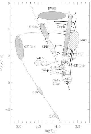
luminosity, falling within instability strips on the Hertzsprung-Russell (HR) diagram. Figure

1.1shows the locations of different classes of variable stars on a HR diagram.

The periodic instability that results in stellar pulsations are caused by internal mechanisms within each star. These mechanisms are known as excitation ordriving mechanismsand are generally a variation of heat-engine mechanisms, first postulated byEddington(1917). Un-like temporary distortions within the stellar interior, which are quickly damped, these mecha-nisms are active and sustained over long temporal periods. In addition, these mechamecha-nisms are cyclical, which means that they incorporate a restoring process that forces a return to equi-librium and keeps the variation regular and stable.

1.3.1

Driving Mechanisms

Three major driving mechanisms for the excitation of pulsations in variable stars have been postulated: theκmechanism, stochastic driving and the εmechanism (Cox, 1980). The κ

mechanism is the most common mechanism producing pulsations in variable stars (Cox,

1980). It operates due to the properties of radiative opacity, denoted by the Greek symbol

κ. Most radial layers or zones of the star prevent or delay radiation (originating in the core) from escaping past those layers (they are partially opaque to radiation). Under compression, some layers become more opaque. This causes those layers to absorb energy, causing the star to expand as a whole, distort the shape of the star or both. However, the chemical elements within those layers (typically hydrogen and helium) become more greatly ionised, decreasing the opacity. This cools those layers and contracts them, forcing them back to and past equi-librium, where they once again become less ionised and more opaque, causing the cycle to repeat.

The second major driving mechanism, operating primarily in the Sun, sun-like stars and some red giants, is stochastic driving (Cox,1980). It is very similar to theκmechanism in that it involves a heat-engine mechanism. However, in the case of stochastic driving, the mecha-nism is not strong enough to produce significant variation on its own. This is due to turbulent

2_{Regular variables are variable stars that show consistent variations in luminosity over a fairly long time period, as}

1.3. Stellar Pulsations

Introduction

Figure 1.1: Locations of different classes of variable stars on a Hertzsprung-Russell (HR) diagram. From Aerts et al.(2010). (Referenced on page3,13,17,18.)

convection currents damping the variation in the inner convective zone (Antoci,2013). In-stead, the oscillations are generated by the resonance of the outer convective zone with the variation in the inner convective zone (Antoci,2013), producing acoustic waves travelling on the surface of the star. This is similar to musical stringed instruments vibrating with their natural frequency in a noisy room.

Introduction

(Cox, 1980). The mechanism relies on variations in the energy generation rate in the core, which can potentially only occur in very massive stars.

In addition to these three major driving mechanisms, there are others such as convective flux blocking3 _{that drive pulsations in certain classes of variable stars. These mechanisms}

tend to be variants of the three major driving mechanisms.

1.3.2

Radial Pulsations

Stellar pulsations can be divided into two main types: radial and non-radial pulsations. Radial pulsations are pulsations in which the entire star expands and contracts with no change in its shape, similar to a balloon into which air is pumped and released. These pulsations are spher-ically symmetric with modes that are characterised by the radial ordern: the number of con-centric nodal shells within each star. Cepheid variables, RR Lyrae stars andδScuti stars (such asHD 3112) are among the types of variable stars exhibiting radial pulsations. Cepheids are

the most ubiquitous examples of radially pulsating stars and tend to pulsate in the fundamen-tal radial mode (Cox,1980). This means that there are no nodal shells within most Cepheids (i.e.n₌0). Instead, the centre of the star functions as a nodal point.

Stars that pulsate in both the fundamental and the first overtone radial modes simultane-ously are particularly useful for asteroseismology. This is because the ratio of the periods of the fundamental and the first overtone in these stars usually differs significantly from those found in stringed instruments (0.5) and in open pipe wind instruments (0.33). For example, this ratio is 0.71 for certain types of Cepheids (Petersen,1973) and 0.78 forδScuti stars ( Pigul-ski et al.,2006). This discrepancy is caused by sound speed gradients within each star, conse-quences of the different internal compositions. Determining the ratio of these modes allows the inference of the internal structures of each star.

1.3.3

Non-Radial Pulsations

Non-radial pulsations are pulsations in which different regions of the star expand and contract at the same time, distorting the spheroidal shape of the star. These pulsations are therefore non-spherically symmetric with modes that are characterised not only by the radial ordern, similar to radial pulsations, but also by the degree`and the azimuthal orderm4<sub>(Aerts et al.,</sub> 2010). The degree`is the total number of nodal lines present on the surface of the star and the azimuthal orderm is the number of nodal lines passing through the poles of the axis of rotation of the star. Technically, radial pulsations also have`andm numbers but these are

3_{Convective flux blocking is a variant of theκmechanism and drives the pulsations inγDoradus stars(Guzik} et al.,2000;Dupret et al.,2004). Refer to the section onγDoradus stars(1.4.1) for more information.

4_{`andmare parameters that describe spherical harmonics. Refer to the section onnon-radial pulsational}

1.3. Stellar Pulsations

Introduction

equal to zero.

Non-radial pulsations can be further subdivided into three types:p-modes,g-modes and

f -modes (Aerts et al.,2010). p-modes are pressure modes, akin to acoustic sound waves and have pressure as their restoring force.g-modes are gravity modes and have buoyancy as their restoring force. f-modes are surface gravity modes, akin to ocean waves but travelling on the surface of the star. The characterisation of a non-radial pulsation mode as either ap-,g- or

f -type aids in the creation and refinement of stellar interior models as these modes penetrate to different depths (Handler,2013).

For example,g-modes penetrate to a greater depth thanp-modes (Handler,2013). There-fore, theseg-modes are indicative of the physical conditions deep within a star and informa-tion such as the size of the stellar core, the interior rotainforma-tion profile and variainforma-tions of the sound speed in the stellar interior can be deduced (Handler,2013). There are also mixed modes: combinations ofp-mode pulsations on the surface and g-mode pulsations in the interior.

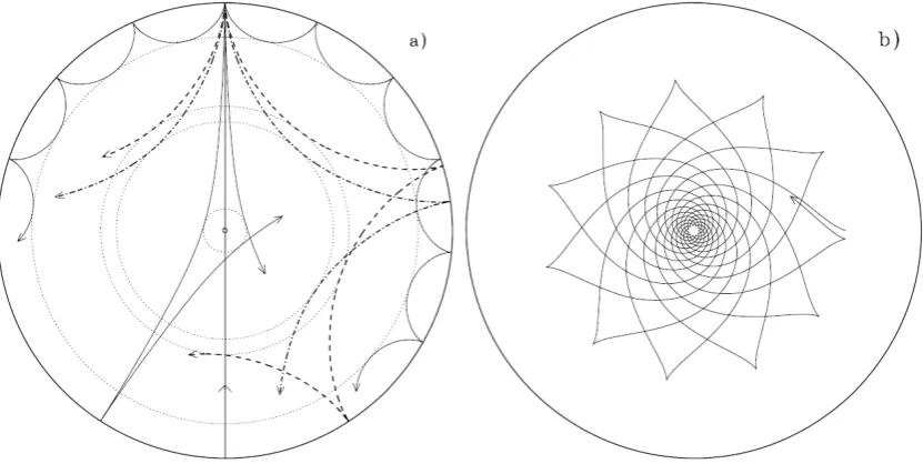
Balona and Evers(1999),Breger and Bischof(2002) andHandler(2005) have found a number ofδScuti starswhich display such modes. Figure1.2shows the propagation ofp-mode and

g-mode waves within a sun-like star.

Introduction

1.3.4

Selection Mechanisms of Pulsation Modes and Frequencies

Although the modes and frequencies of many stars have been identified, a key question that has yet to be definitively answered is this: Why do some stars pulsate with those modes and frequencies? More specifically, why do most Cepheids pulsate in the fundamental radial mode? Why doγ Doradus starsexhibit low frequency g-mode pulsations andδScuti starsexhibit high frequencyp-mode pulsations? What are the selection mechanisms behind modes and frequencies?

Most variable stars show strong fundamental frequency pulsations, similar to musical in-struments, but not all of them. Some classes stars tend to pulsate in specific overtone modes exclusively over others. All of these effects are a result of the physical properties of each star: the location of nodal shells that prevent the excitation of certain modes (Lund et al.,2014), strong magnetic fields that preferentially excite dipole modes (Kurtz et al.,2011), the damp-ing of interior drivdamp-ing forces by the exterior layers (Antoci,2013) and many others (Aerts et al.,

2010). As more information about the interior of the various variable star classes is collated, the question of why certain modes are excited over others might be answered in the future.

1.3.5

Non-Radial Pulsational Geometry

Non-radial pulsations are typically defined in terms of spherical coordinates. The orientation of a star is defined in terms of the inclinationi: the angle between the observer’s line-of-sight and the rotational axis. This parameter is typically unknown or imprecise. Therefore, the rotational velocity is also often not well defined. Instead, the projection of the equatorial ro-tational velocity along the line-of-sight (v sini) is used as a lower bound on the rotational velocity of the star.

Non-radial pulsations are modelled in the programFAMIASas spherical harmonics5that

distort the stellar surface6_{(Zima, 2008b). Spherical harmonics (Y}m

` ) are represented

math-ematically by the product of a trigonometric function (ei mφ_{cosθ) and a Legendre function}

(Pm

` ). The equation defining spherical harmonics is:

Ym ` =N

m ` P

|m|

` ei mφcosθ (1.1)

`is the degree of andm is the azimuthal order (not to be confused with the radial ordern) of the spherical harmonic. θ andφ are the polar and azimuthal angle in spherical coordi-nates. ei mφ_{is the complex exponential form of a trigonometric function (i =}p_{−1 is a}

com-5_{Spherical harmonics are a set of solutions of Laplace’s equation (an equation that describes a scalar field) in three}

dimensions.

6_{Radial pulsations are also modelled inFAMIASusing spherical harmonics but the result is trivial as there is no}

1.3. Stellar Pulsations

Introduction

plex number and not the inclination). Nm

` is a normalisation constant, defined inFAMIAS

(Zima,2008b) as:

Nm

` = (−1)(

m+|m|)/2 v t2`+1

4π

(`_{− |}m_|)!

(`_+|m_|)! (1.2)

The Legendre functions (with respect to the random variablex) are defined by the equation:

P_`m₍x_{) = (−}1₎m₍1₋x2₎m/2 d m

d xmP`(x) (1.3)

P_`(x₎is a Legendre polynomial (not to be confused with a Legendre function), defined by Ro-drigues’ formula as:

P_`(x_{) =} 1

2`<sub>`!</sub>

d` d x`(x

2₋₁ )`

(1.4)

The Legendre function reduces to the Legendre polynomial whenm ₌07_{. The pulsational}

modelling inFAMIASis carried out under the assumption that the rotational axes are aligned

with the coordinate system of the spherical harmonics (i.e. the pulsational axis). Although this is true for most stars (Aerts et al.,2010), it may not necessarily be the case in all stars. For example, in rapidly oscillating Ap (roAp) stars, the pulsation axis is aligned to the magnetic field axis instead of the rotational axis due to the strength of the magnetic field in these stars (Kurtz et al., 2011). There is therefore the possibility that some stars in other variable star classes with strong magnetic fields may exhibit such behaviour as well.

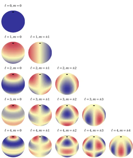
Figure1.3shows a snapshot of various radial and non-radial pulsation modes, up to`<sub>=</sub>4. While the observational identification of high-degree modes using spectroscopy is possible (e.g.Mantegazza and Poretti,2005have identified modes up to`₌16), there are a number of observational and technological difficulties, including insufficient spectral resolution (Balona and Evers,1999;White et al.,2012). In addition, higher-degree modes become progressively more confined to the equatorial region as the azimuthal order increases8 _{(asm approaches} `). This means that modes with both high degree and azimuthal order would be undetectable at low inclinations (close to pole on). Figure1.4illustrates this phenomenon.

The pulsations are also affected by Inclination Angles of Complete Cancellation (IACC)

(Chadid et al.,2001): the inclination angles at which there is a cancellation of the effects of a particular pulsation mode in the stellar spectra. This means that for some inclination angle

i,Pm

` cosi =0. Similarly, one can define Inclination Angles of Least Cancellation (IALC): the

7_P0

`(x) =P`(x)

8_{This phenomenon is due to the nature of the spherical harmonics: whenmapproaches`for large`, the number}

of maxima of|Ym

Introduction

inclination angles at which there is minimal or no cancellation of a particular pulsation mode in the stellar spectra (Pm

` cosi is maximised). An(`,m) = (2,1)mode, for example, hasIACC

at 0◦_{and 90}◦_andIALCat 45◦(Chadid et al.,2001).

Note that these cancellation effects are of the first-order: they only apply to linear quan-tities such as the monochromatic magnitude9_{of photometric data and the radial velocity}10_.

For photometric data that has been recorded with respect to several passbands, which have specific ranges of wavelengths, the comparison of these passbands11_{can mitigate, if not}

to-tally eliminate, the effects ofIACC. In addition, frequency analysis usingthe pixel-by-pixel methodand the higher-order moments of the moment methodwould largely mitigate the effects ofIACC.

1.3.6

Rotational Effects on Pulsations

Stellar pulsations can be most significantly affected by the rotations of the stars about their axes (García et al.,2014). This is because the pulsations distorting the surfaces of the stars are affected by changes in the geometry of the star12_{. Although other factors, such as turbulence}

and granulation13_{, affect stellar pulsations, they are considered to be relatively minor in}

com-parison with rotational effects. In addition, current understanding of such effects is limited (Gray,1975,1988,2005). As such, these more minor effects will not be taken into account for the purposes of this thesis.

m₌0 modes are known as axisymmetric modes as the locations of the nodal lines are sym-metric about the pulsation axis, which is assumed to be aligned with the rotation axis14_{. These}

modes are standing waves and are therefore unaffected by rotation15_{. m 6}

=0 modes are trav-elling waves and are divided into two groups: prograde modes (m>0) and retrograde modes (m <0)16_{. Prograde modes travel along the direction of rotation while retrograde modes travel}

opposite to the direction of rotation. This is of particular concern when the pulsational and

9_{The monochromatic magnitude is an absolute measure of the brightness of a star across a passband. It is defined}

as the logarithm of the spectral flux density. Refer toOke and Gunn(1983) for more information.

10_{The radial velocity is equivalent to the first moment of the Moment Method (Aerts,1996). Refer to the section on}

the moment method(2.4.1) for more information.

11_{SinceIACConly affects the monochromatic magnitude, taking the amplitude ratios of different passbands}

would eliminate the dependence oni. Refer toAerts et al.(2010) for more information.

12_{Refer toAerts et al.(2010) for a definitive list of rotational effects and their mathematical and physical}

founda-tions.

13_{Turbulence is the mathematically chaotic flow of a fluid. Granulation is the conglomeration of fluid particles due}

to viscosity. Both of these phenomena work in conjunction, producing asymmetries and other minor variations in stellar spectral lines. Refer toGray(1975,1988,2005) for more information.

14_{Refer to the section onnon-radial pulsational geometry(1.3.5) for more information.}

15_{Note that this definition assumes that the star does not deviate from spherical symmetry at equilibrium, which}

is generally untrue (stars exhibit varying amounts of rotational flattening). Refer toReese et al.(2006) for more information.

16_{Note that the sign convention for prograde and retrograde modes may be reversed in other papers (e.g.}

1.3. Stellar Pulsations

Introduction

rotational periods are similar to each other, as is the case forγDoradus stars.

`₌2,m_=±1

`₌1,m_=±1

`₌1,m ₌0

`₌0,m ₌0

`₌2,m ₌0

`<sub>=</sub>3,m <sub>=</sub>0 `₌3,m_=±1 `₌3,m_=±2

`₌2,m_=±2

`₌3,m_=±3

`₌4,m_=±3

`₌4,m_=±2

`₌4,m_=±1

`<sub>=</sub>4,m <sub>=</sub>0 `₌4,m_=±4

Figure 1.3: Radial and non-radial pulsation modes of a star at an inclination of 60◦. These diagrams are the mapping of spherical harmonics onto the surfaces of spheres, with no consideration of rotational effects. The north poles are represented by black ellipses. The degree`and the azimuthal orderm

Introduction

`₌20,m_=±5

`<sub>=</sub>20,m<sub>=</sub>0 `₌20,m_=±10 `<sub>=</sub>20,m<sub>=±</sub>15 `₌20,m _=±20

Figure 1.4:`=20 pulsation modes of a star at an inclination of 60◦. These diagrams are the mapping of spherical harmonics onto the surfaces of spheres, with no consideration of rotational effects. The north poles are represented by black ellipses. The degree`and the azimuthal ordermof each mode has been printed above each diagram. The yellowish-white lines are the surface nodes while the red and blue areas represent the regions of the star that are moving inwards (or outwards) or cooling (or heating) at a particular time. Note the progressive confining of the pulsation to the equatorial region as|m|increases. (Referenced on page8,12.)

The main structural effect of rotation is the deviation of the pulsationally unperturbed star from spherical symmetry due to rotational flattening. This means that the modelling of stellar pulsations as a single spherical surface harmonic becomes imprecise (Reese et al.,2006). Un-fortunately, there are currently no asteroseismological surface models taking this factor into account.

Rotational splitting is another effect of rotation. This phenomenon causes the prograde orders of a mode with a certain`to have higher frequencies and the retrograde orders to have lower frequencies. This is due to simple vector addition: the rotational frequency vector is added to the pulsational frequency for the case of prograde modes and subtracted from the pulsational frequency for the case of retrograde modes (Aerts et al.,2010). Note that the Cori-olis force opposes this phenomenon: the frequency of prograde modes are reduced while the frequency of retrograde modes are increased. However, the effects of the Coriolis force is much weaker than the effects of rotational splitting for stars with slow to medium rotational veloc-ities (Saio,2013). The increase or decrease in frequency varies according to the order of the mode, causing any one frequency to be split into a total of 2`₊1 frequency multiplets.

However, most stars exhibit differential rotation17_{(Gizon and Solanki, 2004;Lund et al.,} 2014), implying that the splitting process is complicated and non-uniform. The inclination of the star would therefore influence the number of detected multiplet components. In addition, different multiplets are excited to different amplitudes depending on the physical conditions of the star (Miesch,2005; Lund et al.,2014). Some components may therefore not even be detectable due to the low amplitudes. Comparing the multiplets of modes with different`or

17_{Differential rotation is the rotation of different latitudinal regions of a star at different speeds. This is in contrast}

1.3. Stellar Pulsations

Introduction

n values18_{enable the measurement of the interior rotation rate of the star}19_{(Benomar et al.,} 2015).

A recent study byChapellier et al.(2012), usingCoRoTphotometry, showed some

evi-dence that space-based photometry is precise enough for the identification of split frequen-cies inγDoradus starsandδScuti stars. However,Chapellier et al.(2012) mentioned that the origins of the frequency splitting was highly uncertain and that the star that they had analysed (CoRoTID 105733033) could possibly be a binary. In addition, the plethora of identified

fre-quencies, many of which are potential aliases, harmonics or combinations thereof20_{, made}

identification of frequency multiplets difficult and imprecise.

Another recent study byBouabid et al.(2013) proposes an origin for mixed modes21_inγ Doradus starsand δ Scuti stars. They discovered that frequencies between those typically exhibited by the two classes of stars can be explained by the rotational shifting of prograde

g-modes inγDoradus stars to higher frequency values.

It has been theorised byTownsend(2003b) that prograde tesseral modes22_{of rapidly-rotating}

stars have reduced photometric amplitudes. This is because the pulsations become increas-ingly confined to the equatorial region as the rotational velocity increases, due to increasing Coriolis force. This phenomenon is independent of the confining of high-order, high-degree modes to the equatorial region23_{(Figure1.4) and as such, applies to pulsations of all degrees}

and azimuthal orders. This means that some of the pulsation modes of rapidly-rotating stars with low inclinations would not be detectable photometrically (Townsend,2003a,b) or spec-troscopically (Townsend,1997,2003a;Daszy´nska-Daszkiewicz et al.,2007).

1.3.7

Pulsational Effects on Spectroscopic Data

Radial and non-radial pulsations manifest as asymmetric deviations across the spectral lines of a stellar spectrum. These are the result of the minute radial velocity and temperature vari-ations caused by the expansion and contraction of the outer layers of the star. There is a small blueshift in radial velocity when there is expansion and small redshift in radial velocity when there is a contraction along the along the observational line-of-sight. One would also expect the spectroscopic variations to also typically correspond to the photometric variations, but

18_{Some asteroseismological analysis software packages, likeTOUCAN(Rodrigo et al.,2015;Suárez et al.,2014),}

allow for the measurement ofnvalues.

19_{The interior regions (core and radiation zone) of stars are considered to rotate uniformly (as rigid bodies) (}

Beno-mar et al.,2015). This was first observed in the Sun (refer toGaraud,2002;Garaud and Garaud,2008; Acevedo-Arreguin et al.,2013for detailed reviews).

20_{Refer to the section onfrequency identification(2.4.1) for more information.} 21_{Refer to the section onnon-radial pulsations((1.3.3) for more information} 22_{Tesseral modes are modes where|m| 6}

=`. Prograde tesseral modes are therefore modes where` >m>0.

Introduction

this does not always seem to be case24_{(Balona,1998).}

The spectra in this analysis are reduced to cross-correlated line profiles25_{for ease of}

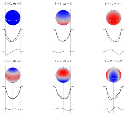
anal-ysis and to increase the signal-to-noise ratios of the individual spectra. Figure1.5shows how different pulsation modes distort the shape of the cross-correlated line profiles. The frequen-cies of these variations are then identified using Fourier analysis and the line profile variations are then modelled as functions of the`andm values of various modes usingFAMIAS26. As

mentioned in the preceding sections, these models are reasonably idealised and do not take into account many physical factors, such as rotational flattening. However, it is assumed that these models are a reasonable approximation for non-radially pulsating and slowly rotating stars.

1.4

Variable Star Classes

1.4.1

γ

Doradus Variable Stars

γDoradus variable stars were first suggested as a new class byKrisciunasin1993. They were named after the prototypical starγDoradus, whose variability was first discovered byCousins and Warren(1963) and later analysed byCousins et al.(1989). Kaye et al.(1999) andPollard

(2009) are the two most recent reviews ofγ Doradus stars and the theoretical and observa-tional challenges faced when analysing such stars.

As of 2011, there were 86 bright bona fide γDoradus stars (Henry et al., 2011), most of whose variability was originally found through the Hipparcos mission (Perryman et al., 1997;Aerts et al.,1998;Waelkens et al.,1998;Eyer and Aerts,2000). 418 candidates had been identified byCoRoT(Hareter,2012) and 207 byKepler(Uytterhoeven et al.,2011;Bradley et al., 2015). TheMOST satellite has been used for follow up work on some of these stars,

primarily collecting long timebase photometric data (Rowe et al., 2006; Sódor et al., 2014). The number of bona fide members is expected to rise significantly with the first data release (mid-2016) from the recently-launchedGaiamission, currently the most advanced space

ob-servatory in orbit.

γDoradus stars are typically Population I27_{, late A- to early F-type stars. They are}

charac-terised by theirg-mode pulsations of highn and low`28(Kaye et al.,1999). These stars have

24_{Refer to the sections onnon-radial pulsational geometry(1.3.5) and therotational effects on pulsations(1.3.6)}

for more information on exceptions to this rule.

25_{Refer to the section oncross-correlation(2.2.3) for more information.}

26_{Refer to the section onspectroscopic variability analysis(2.4) for more information on the frequency and mode}

identification process.

27_{Population I stars, one of the two “populations” of stars originally defined byBaade(1944), are generally young}

stars with high metallicity.

28_{Refer to the sections onnon-radial pulsations(1.3.3) andnon-radial pulsational geometry(1.3.5) for more}

1.4. Variable Star Classes

Introduction

`<sub>=</sub>0,m<sub>=</sub>0 `₌1,m₌0 `₌1,m₌1

`<sub>=</sub>2,m<sub>=</sub>0 `₌2,m₌1 `₌2,m₌2

Figure 1.5: An animated diagram showing the line profile variations of various modes due to pulsations. The degree`and the azimuthal ordermhave been printed above each diagram. The top panels of each diagram are the spherical harmonics, the middle panels are the distorted cross-correlated line profiles and the bottom panels are graphs showing the variation of each line profile from a pulsationally unper-turbed line profile (assumed to be Gaussian). The animations can be viewed in Adobe Reader. Anima-tions obtained from Dr. John Telting’s website (http://staff.not.iac.es/~jht/science/ nrpform/). (Referenced on page13.)

typical frequencies between 0.3 d−1_{and 3 d}−1_{with luminosity variations of up to 0.1}

magni-tudes and radial velocity variations of up to several kilometres per second (Guzik et al.,2000). The frequencies ofγDoradus stars are much smaller than those of the fundamental radial modes of A- to F-type stars, which are between 8 d−1_{and 24 d}−1_{. They are located along the}

intersection between the classical instability strip and the main sequence branch of the HR diagram (Figure1.1).

Introduction

magnitude above theZAMS(Handler,1999).Henry et al.(2011) observed that stars belonging

to both subgiant (IV) and dwarf (V) luminosity classes could exhibitγDoradus-like pulsations and found that approximately 22% of A7- to F5-type stars of their sample of 114 stars were bona-fideγDoradus stars. γDoradus stars have typical masses of about 1.51 Mto 1.71 M and typical radii of about 1.43 Rto 2.36 R(Kaye et al.,1999).

It was first theorised byGuzik et al.(2000), using frozen convection models, that the driving mechanism behind the pulsations ofγDoradus stars was convective flux blocking (Pesnell,

1987), a variant of theκ-mechanism29_{. Dupret et al.(2004) later expanded upon the proposal}

ofGuzik et al.(2000) using a time-dependent treatment of convection, producing instability strips forγDoradus stars of various masses and luminosities (refer to Figure1.6).Dupret et al.

then refined their models in2005and used them to predict the photometric behaviour of five of the most well-studiedγDoradus stars (Dupret et al.,2005b).

γDoradus stars have a three-layer internal structure: a convective core, an intermediate radiative zone and an outer convective envelope (Guzik et al.,2000). The pulsations in the ra-diative zone, arising because of opacity variations, attempt to propagate to the outer regions through radiative heat transfer. However, the convective envelope is resistant to the radiative heat transfer from the interior, resulting in a blockage of radiative flux by the convective enve-lope (Pesnell,1987). The degree of blockage varies periodically, driving the pulsations in the interior of the star. Theg-mode pulsations inγDoradus stars arise due to this mechanism (Dupret et al.,2006).

γDoradus stars have been studied quite extensively. Detailed photometric and spectro-scopic frequency and mode identifications of stars such as HD 12901 (Brunsden et al.,2012), HD 135825 (Brunsden,2013), HD 139095 (Greenwood,2014), HR 8779 (Sódor et al.,2014) and KIC 6462033 (Ulusoy et al.,2014) have been performed. All of the aforementioned stars were reported to display the low frequencies and low degree modes typical ofγDoradus stars. How-ever, some stars such as CoRoT ID 105733033 (Chapellier et al.,2012), BD+18 4914 (Rowe et al.,

2006) and KIC 9533489 (Bognár et al.,2015) were also reported to display high-frequency pul-sations in addition to the low-frequency pulpul-sations30_{. Further investigation ofγDoradus stars}

would be useful to determine the origin of the high frequency variation in certainγDoradus stars.

29_{Refer to the section ondriving mechanisms(1.3.1) for more information}

30_{These stars are referred to asδScuti-γDoradus hybrids. Refer to the section onδScuti stars(1.4.2) for more}

1.4. Variable Star Classes

Introduction

Figure 1.6: TheoreticalγDoradus instability strips for stars vibrating with`=1 modes. The thick solid lines denote the instability strips at different values of the mixing-length parameterαa. The thin dashed lines denote the results using the less sophisticated frozen convection model ofWarner et al.(2003). The circles represent bona fideγDoradus stars. The dotted lines denote isochrones at the various masses indicated on the right edge of the diagram. FromDupret et al.(2004). (Referenced on page15, 18.)

Figure 1.7: TheoreticalδScuti instability strips for stars vibrating with`=2 modes. p,g andf repre-sent the type of mode (either pressure, gravity or surface gravityb_{), the subscripted number represents} the order of the mode and the subscriptsRandBrepresent the red and blue edges (arbitrarily defined) of the mode. The points represent observedδScuti stars. The solid lines extending from left to right denote isochrones at the various masses indicated on the right edge of the diagram. FromDupret et al. (2004). (Referenced on page18.)

a_{The mixing-length parameter is the ratio that represents the degree of coherence of a fluid globule (which forms} due to viscosity of the fluid) in fluid dynamics.

Introduction

1.4.2

δ

Scuti Variable Stars

δScuti stars are a well-established class of variable stars, first defined byEggenin1956. They are named after the prototypical star,δScuti, whose variability was first discovered by Camp-bell and Wright(1900). The photometric variability and radial velocity variations were first characterised byFath(1935) andColacevich(1935) respectively, more than thirty years after the discovery of the star.Breger(2000),Lampens and Boffin(2000) andRodríguez and Breger

(2001) had published reviews on theδScuti class, withLampens and Boffin(2000) focussing specifically on those present in multi-star systems.

Being such a well-established class, more than 1500 bona fide members and several thou-sand candidates have been identified and catalogued (Rodríguez et al.,2000;Rodríguez and Breger,2001;Balona and Dziembowski,2011). Large quantities of follow-up work has been carried out using satellite data. Analysis ofWIREdata has shown that the bright star Altair,

also known asαAquilae, is aδ Scuti star, and the brightest one discovered to date (Buzasi et al., 2005). Data from MOST(Breger et al., 2012b), CoRoT (Kaiser et al., 2009) and Ke-pler(Bradley et al.,2015), have also been used in a number of in-depth studies on

individ-ual members: Rho Puppis (Antoci et al.,2009), HD 174936 (García et al.,2009), KIC 9700322 (Breger et al.,2011), KIC 80541466 (Breger et al.,2012a) and HD 261711 (Zwintz et al.,2013). HD 261711 and KIC 9700322 were reported to display low-degree (` <3) non-radial modes. Rho Puppis was also reported to display solar-like pulsations in addition to a dominant ra-dial pulsation mode. KIC 8054146 was also reported to display low frequencyg-modes and and high frequencyp-modes. All of the aforementioned stars were also reported to display regularities in the spacings between identified frequencies.

δScuti stars are typically Population I31_{, early A- to early F-type stars. They are}

charac-terised by both radial pulsations andp-mode pulsations of low`32 (Rodríguez and Breger,

2001). These stars have typical frequencies between 3 d−1 _{and 80 d}−1 _{with a wide range of}

luminosity variations: anywhere from 0.001 to 1 magnitude (Rodríguez and Breger, 2001). They are located along the intersection between the classical instability strip and the main sequence branch of the HR diagram (refer to Figure1.1), similar toγDoradus stars.

δScuti stars tend to have spectral types between A2 and F5 and may belong to giant (III), subgiant (IV) and dwarf (V) luminosity classes (Rodríguez and Breger, 2001). Breger(2000) had estimated that approximately 30% of all A2- to F5-type stars could exhibitδ Scuti-like pulsations.δScuti stars have typical masses of about 1.5 Mto 2.5 M(Aerts et al.,2010).

δ Scuti stars that pulsate with large luminosity amplitudes are grouped into a subclass called High Amplitude Delta Scuti (HADS) stars. Those which pulsate with low luminosity

31_{Refer to the section onγDoradus stars(1.4.1) for more information.}

32_{Refer to the sections onnon-radial pulsations(1.3.3) andnon-radial pulsational geometry(1.3.5) for more}

1.4. Variable Star Classes

Introduction

amplitudes are similarly grouped into a subclass called Low Amplitude Delta Scuti (LADS)

stars. HADS stars were initially thought to be monoperiodic and hence not too useful for

asteroseismology33_{. They were observed to pulsate most strongly in the fundamental radial}

mode, with typical frequencies of between 8 d−1 _{and 24 d}−1_{for A- to F-type stars. This was}

refuted by Mathias et al.(1997), who had managed to discover non-radial modes using ra-dial velocity measurements. Poretti(2003) later attributed the variation in the light curves ofHADSto non-radial pulsation modes. According to a theoretical model developed byLee et al.(2008), only 0.3% ofδScuti stars are expected to beHADSstars, while more than 33%

are expected to beLADSstars.

Another interesting subclass that has been defined in recent years is theδScuti-γDoradus hybrid: stars displaying high-frequencyp-mode pulsations, characteristic ofδScuti stars, as well as low-frequencyg-mode pulsations, characteristic ofγDoradus stars. Researchers in-cludingRowe et al.(2006),Chapellier et al.(2012),Hareter(2012),Brunsden(2013) andBognár et al.(2015) have conducted detailed analyses of stars within this subclass. Recent results from the analysis ofKepler data (Balona,2014) has revealed a surprising claim: allδScuti stars

display low-frequency pulsations. Balona et al.(2015) conducted detailed modelling of the hybrid stars and concluded that the low-frequency pulsations could not be attributed to rota-tional effects or anomalous chemical compositions. This means that the concept of a hybrid pulsator would become meaningless: the pulsational characteristics of theδScuti class may need to be redefined to includep-,g and mixed-mode non-radial pulsations of both low and high frequencies.

Dupret et al.(2004) computed theoreticalδScuti instability strips for stars of various masses and luminosities (refer to Figure1.7) using a time-dependent treatment of convection. In con-junction with Figure1.6, it can be observed that there is a large degree of overlap between the

γDoradus andδScuti instability strips that is not visible in Figure1.1. This was further ex-tended byMontalbán and Dupret(2007), who incorporated turbulence34_{into the pulsational}

modelling. There is strong evidence that thep-mode pulsations inδScuti stars are driven by theκmechanism35_{, particularly in the second partial ionisation zone of helium. The origin of}

theg- and mixed-modes inδScuti stars is currently unknown (Balona et al.,2015). The new revelations ofBalona(2014) andBalona et al.(2015) necessitate additional investigation into the relationship betweenγDoradusandδScutistars.

33_{Refer to the section onradial pulsations(1.3.2) for more information}