PATIENT SAFETY
Experimental Study and Optimization of Scan
Parameters That Influence Radiation Dose in
Temporal Bone High-Resolution Multidetector
Row CT
Y.T. Niu M.E. Olszewski Y.X. Zhang Y.F. Liu J.F. Xian Z.C. Wang
BACKGROUND AND PURPOSE:MDCT has some specific scan parameters that may systematically
increase or decrease radiation dose to patients. This study explored the scan protocol parameters that impact radiation dose in temporal bone MDCT and determined the optimal scan parameters that balance radiation dose with diagnostic image quality.
MATERIALS AND METHODS: Using exsomatized cadaveric heads, traditional axial scanning, and helical scanning were performed with different detector collimations. Helical scans of the same scan region were then acquired by using the determined optimal detector collimation and various tube voltages, whereas other scan parameters remained fixed. Next, the scans were repeated by using various tube current-time products by using the determined optimal tube voltage. Last, with fixed tube current-time product, the scans were repeated with various pitches. All thin-section, helically acquired scans were reformatted to axial and coronal images with respect to the relevant scanning baseline. In each of the image volumes, the mean and SD HU values in regions of interest were measured in the central section of the internal auditory canal, and CNR values were calculated.
RESULTS: In agreement with theory, wider detector collimations such as 16⫻0.625 mm and 64⫻ 0.625 mm were associated with lower radiation doses than narrower collimations due to their lower overbeaming and higher geometric efficiency. In helical scanning, the detector collimation of 16⫻0.625 mm had higher image quality and the minimum DLP. Axial and coronal images acquired by using a 140-kVp tube voltage had significantly lower noise than scans acquired at 120 or 80 kVp with equivalent volume CT dose index. Diagnostic image quality was achieved when using a minimum tube current-time product of 120 mAs. Noise, CNR, and dose were jointly optimized with a pitch of 0.685.
CONCLUSIONS:Temporal bone CT scanning parameters may be optimized by following a systematic procedure that allows for the optimization of diagnostic image quality and the minimization of radiation dose. One such procedure for a particular 64-section MDCT scanner has been presented.
ABBREVIATIONS:CNR⫽contrast-to-noise ratio; CTDIvol⫽volume CT dose index; DLP⫽ dose-length product; HU ⫽ Hounsfield Unit; kVp ⫽ peak kilovoltage; mAs⫽ current-time product; MDCT⫽multidetector row CT; ROI⫽region of interest
I
n recent years, CT technology has undergone profound changes. Compared with single-section CT, MDCT has some specific scan parameters that may systematically increase or decrease radiation dose to patients, while enabling the vi-sualization of the microanatomic structures of the temporal bone.1There is potential for dose reduction with MDCT sys-tems, but the actual dose reduction achieved depends upon how the system is used. There is increasing awareness of how adapting exposure factors, such as overranging, overbeaming, tube voltage (kVp), effective mAs, pitch, and scan length, can contribute to the management of patient dose. In this study, the scan parameters that affect radiation dose in temporal bone MDCT were investigated, and the combination ofpa-rameters with the lowest radiation dose yielding diagnostic image quality were determined.
Materials and Methods
Subjects
Four exsomatized cadaveric heads were included in the study. The cadaveric heads were removed from storage in formalin solution and positioned upright approximately 12 hours before scanning to dis-charge the solution from the nasal cavity and external auditory canal. A pilot study of the 4 heads was performed to select the head most fit for the experiment.
CT Technique
All the images in this study were acquired by using a 64-channel MDCT scanner (Brilliance; Philips Healthcare, Cleveland, Ohio) by using various scanning modes and parameter settings. The direct axial images were acquired with the subject’s neck flexed and the gantry angled in the cranial direction so that the skull base (ie, the glabel-lomeatal line) was parallel to the scanning plane. No gantry angula-tion was used for helical scanning; the cadaveric head was placed on the table with the scanning baseline parallel to the acanthiomeatal Received September 21, 2010; accepted after revision February 15, 2011.
From the Department of Radiology (Y.T.N., Y.X.Z., Y.F.L., J.F.X., Z.C.W.), Beijing Tongren Hospital, Capital Medical University, Beijing, China; and Philips Healthcare (M.E.O.), Cleveland, Ohio.
Please address correspondence to ZhenChang Wang, MD, Department of Radiology, Beijing Tongren Hospital, Capital Medical University, No. 1 Dongjiaominxiang, Dongcheng District, Beijing 100730, China; e-mail: [email protected] or [email protected]
http://dx.doi.org/10.3174/ajnr.A2609
PATIENT
line.2The following sections detail the steps that were taken to deter-mine the optimal temporal bone scanning protocol parameters.
Axial Scanning with Different Detector Collimations
In MDCT, the craniocaudal dose profile takes the form of a trapezoid due to the x-ray path from source to detector. Although the central plateau of the trapezoid, or umbra, of the dose profile may be used for image reconstruction, the triangular ends of the trapezoid, also known as the x-ray penumbra, cannot be used for image reconstruc-tion due to incomplete illuminareconstruc-tion of all detector elements.3 Over-beaming is when the x-ray beam incident on the patient extends be-yond the active detector area and hence part of the beam is not used for imaging purposes. The dose is largest when the total beam width is small. Generally, wider beam collimation in MDCT results in more dose-efficient examinations, because overbeaming constitutes a rela-tively smaller proportion of the detected x-ray beam. But, if the small anatomic area of the temporal bone is scanned, the specific scan length and overbeaming should both be taken into account except other dose-influencing factors such as overscanning while selecting the optimal collimation width. In this study, conventional direct axial CT scans were performed with a tube voltage of 140 kVp and a tube current-time product of 180 mAs/section. Scanning was repeated with the various detector collimations available on the system for axial scanning (ie, 2⫻0.625, 12⫻0.625, 16⫻0.625, 40⫻0.625, and 64⫻ 0.625 mm). Images were reconstructed with a 1.25-mm section thick-ness and a 1.25-mm section interval.
Helical Scanning with Different Detector Collimations
In addition to overbeaming, overscanning results from helical or axial acquisitions where the x-ray exposure at the start and end of each scan exceeds the planned scan length. Although unnecessary radiation can occur at either or both ends of a planned acquisition due to subopti-mal scan planning by the CT technologist or physician, overscanning also is associated with the scanner design and may result even when scan ranges are optimally planned. In helical scans this overscanning, also known as overranging, is due to extra gantry rotations necessary to gather sufficient x-ray projection data for image reconstruction and results in an irradiated craniocaudal length that exceeds the dis-tance between the first and last reconstructed image sections. Com-bined with the results in axial scanning with different detector colli-mations, helical scans were performed with a tube voltage of 140 kVp, a tube current-time product of 180 mAs/section, and a pitch of 1.0 to find the appropriate collimation for temporal bone spiral CT. Scan-ning was repeated with the different detector collimations available on the system for helical scanning (ie, 2⫻0.5, 16⫻0.625, 20⫻0.625, 40⫻0.625, and 64⫻0.625 mm).
Helical Scanning with Different Tube Voltages
Tube voltage determines the energy distribution of the incident x-ray beam. Variation in the tube voltage causes a substantial change in CT
dose, as well as image noise and contrast. Using the axial and helical datasets acquired with the aforementioned protocols, the optimal de-tector collimation was determined. After the determination of the detector collimation, we examined the effect of tube voltage. Axial and helical scans were then performed by using tube voltages of 80, 120, and 140 kVp, with a pitch of 1.06. To keep CTDIvolconstant among the scanning protocols, tube current-time products of 540 (the closest value to 551 mAs/section that could be selected), 240, and 180mAs/section were used for each tube voltage, respectively.
Helical Scanning with Different Effective Tube Current-Time Products
With the previously determined optimal detector collimation and tube voltage, various effective tube current-time products (ie, 40, 80, 120, 160, 200, 240, 280, 320, and 360 mAs/section) were evaluated for helical scanning with a pitch of 1.06 to determine the most appropri-ate effective mAs with the resulting image quality meeting the diag-nostic requirements.
Helical Scanning with Different Pitches
Finally, by using the identified optimal detector collimation, tube voltage, and effective tube current-time product, various pitches (ie, 0.19, 0.31, 0.44, 0.685, 0.935, 1.19, and 1.315) were evaluated to find the pitch suited for temporal bone CT.
Image Reconstruction and Reformation
For all scans, a high-resolution dataset was reconstructed by using an enhanced Y-sharp (C) reconstruction kernel with an edge-enhance-ment factor of 1 and a transaxial FOV of 20 cm. All images were reconstructed on a 512⫻512 matrix at a thickness of 0.67 mm with 0.33-mm overlap. All helically acquired, thin section images were reformatted into axial and coronal images with 1-mm thickness and 1-mm increment by using a dedicated postprocessing workstation (Extended Brilliance Workspace; Philips Healthcare).
Image Quality Evaluation
Subjective Assessment.Two senior radiologists and 1
technolo-gist graded the image quality of the reformatted images by using a 3-point ordinal scale. An image quality of grade I was excellent, with no diagnostic limitations; grade II was of lower quality but did not affect the diagnosis; and grade III was very low quality and may have influenced the diagnosis. Grade I and grade II images were considered to be of diagnostic image quality.
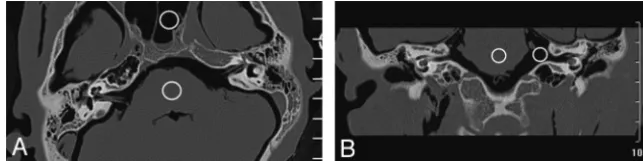
Objective Measurement.The mean and SD HU values in the
ROIs shown in Fig 1 were measured. The CNR of each image was calculated by the following equation:
CNR⫽ Mbrain stem⫺Mair
冑
SDbrain stem2 ⫹ SDair2 2 [image:2.594.132.454.44.124.2]Radiation Dosimetry
The CTDIvolfor each scan was measured by using a dedicated dosim-eter (CT Dose Profiler; RTI Electronics, Mo¨lndal, Sweden) and re-corded. The DLP for each scan was calculated by using the measured CTDIvoland the scan length.
Results
Image Quality and Radiation Dose Variations with Detector Collimation in Axial Scanning
The CTDIvol, DLP, noise, and CNR of axial images for each detector collimation are shown in Table 1.
Image Quality and Radiation Dose Variations with Detector Collimation in Helical Scanning
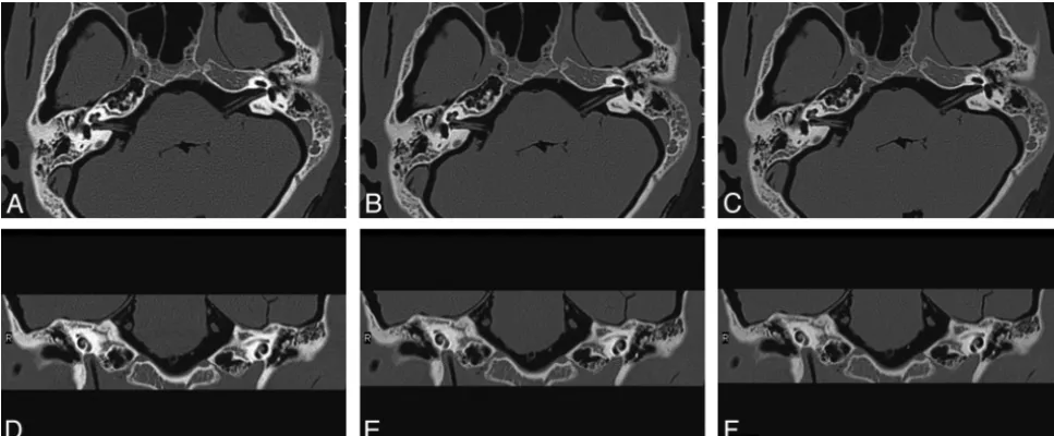
The CTDIvol, DLP, noise, and CNR of axial and coronal im-ages reformatted from helical acquisitions with each detector collimation are shown in Table 2.
Image Quality and Radiation Dose Variations with Tube Voltage in Helical Scanning
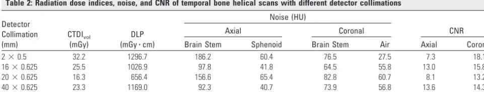
Examples of axial and coronal images reformatted from helical acquisitions with each kVp are shown in Fig 2. The CTDIvol, DLP, noise, and CNR of each acquisition are shown in Table 3.
Image Quality and Radiation Dose Variations with Effective Tube mAs in Helical Scanning
The CTDIvol, DLP, noise, and CNR of axial and coronal im-ages reformatted from helical acquisitions with each effective tube mAs are shown in Table 4. Table 5 lists the ordinal image quality scores of the reformatted images as rated by the 3 observers.
Image Quality and Radiation Dose Variations with Pitch
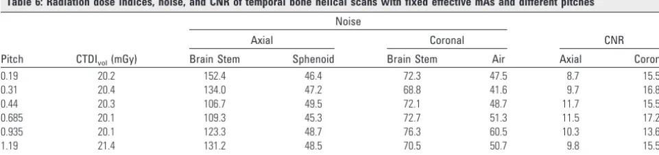
The CTDIvol, noise, and CNR of axial and coronal images re-formatted from helical acquisitions with fixed effective mAs of 200 and each pitch are shown in Table 6.
Discussion
Two sources of undesired patient radiation exposure exist in the z-axis direction in MDCT: overbeaming3and overscan-ning.4Overbeaming is defined as the penumbto-umbra ra-tio, and it degrades the geometric dose use of a scanner,3,5thus exposing a patient to unnecessary radiation; however, wider detector collimations lead to a smaller penumbra-to-umbra ratio and higher geometric dose use.6,7In contrast to over-beaming, the effect of overscanning increases with the increas-ing cone angle of large-coverage MDCT scanners and contrib-utes a larger proportion of the total effective dose for small craniocaudal scan lengths, such as those associated with tem-poral bone imaging.
[image:3.594.52.285.71.154.2]In axial imaging, the 2⫻0.625-mm detector collimation had more overbeaming, yielding a geometric dose use of only 37%. Therefore, with the same scanning parameters, the CTDIvol with the 2 ⫻ 0.625-mm detector collimation in-creased to 47.2 mGy as shown in Table 1, approximately 2 times the CTDIvol of the other collimations. The 40 ⫻ 0.625-mm detector collimation provided the best balance among CTDIvol, noise, and CNR; however, the 25-mm cover-age of the 40⫻ 0.625-mm detector collimation required 2 rotations to completely image the temporal bone, resulting in an imaged length of 50 mm. In clinical practice, a scan length of 40 mm is typically used to image the temporal bone. The coverage of the 16⫻ 0.625- and 64⫻0.625-mm detector collimations was 20 and 40 mm, respectively. Thus, the anat-omy could be imaged with 1 or 2 rotations, respectively. As a result of the 10 mm of overscan (50-mm scan length versus 40-mm anatomic extent), the DLP associated with the 40⫻ 0.625-mm detector collimation was 34% higher than the DLP associated with the 16⫻0.625-mm detector collimation and 56% higher than the 64⫻0.625-mm detector collimation. To this end, the 64⫻0.625-mm detector collimation resulted in the lowest overall dose for the examination, though the noise was slightly higher and the CNR slightly lower, respectively, than the 40⫻0.625-mm detector collimation. Nevertheless, it should be noted that the noise and CNR differences between the 64⫻0.625- and 40⫻0.625-mm detector collimations may be less than the differences in the same metrics among subjects in practice, and may reflect the limited sample size in Table 1: Radiation dose indices, noise, and CNR of temporal bone
axial scans with different detector collimations
Detector Collimation (mm)
CTDIvol
(mGy)
DLP
(mGy䡠cm)
Noise (HU)
CNR
Brain Stem Sphenoid
2⫻0.625 47.2 1898.6 77.9 41.4 16.1 12⫻0.625 20.8 935.6 18.7 15.0 60.5 16⫻0.625 22.6 902.8 82.9 43.4 15.1 40⫻0.625 24.2 1211.5 75.3 34.6 17.2 64⫻0.625 19.4 775.6 80.4 49.6 14.8 Note:—When the 12⫻0.625-mm collimation was selected, the system could not choose 180 mAs/section. The closest tube mAs, 165 mAs/section, was selected. In addition, the 12⫻0.625-mm collimation used the system’s “detailed resolution” setting and got substantially different noise and CNR, with no comparability with other collimations. The 12⫻0.625-mm detector collimation was not available in helical mode and was not included in the comparison.
Table 2: Radiation dose indices, noise, and CNR of temporal bone helical scans with different detector collimations
Detector Collimation (mm)
CTDIvol
(mGy)
DLP
(mGy䡠cm)
Noise (HU)
CNR
Axial Coronal
Brain Stem Sphenoid Brain Stem Air Axial Coronal
2⫻0.5 32.2 1296.7 186.2 60.4 76.5 27.5 7.3 18.1
16⫻0.625 25.5 1026.9 97.8 41.8 64.5 55.8 13.0 15.8
20⫻0.625 16.3 656.4 156.6 65.4 82.8 60.7 8.1 13.2
40⫻0.625 23.3 1169.0 92.3 40.7 73.9 56.8 13.6 14.3
64⫻0.625 22.9 1836.6 99.9 45.9 62.7 60.5 12.3 15.6
[image:3.594.52.533.620.712.2]this study. In contrast, one would not expect the dose to vary from subject-to-subject with the same protocol parameters.
Overbeaming and overscanning also occur in helical scan-ning, though they differ in the relative degree that they influ-ence radiation dose. Overbeaming has a detrimental effect on geometric dose use, particularly at narrower detector collima-tions such as 2⫻0.5 mm. The higher proportion of over-beaming at this collimation resulted in a substantially higher CTDIvolthan the CTDIvolfrom other detector collimations with the same effective tube mAs. In helical MDCT, overscan-ning caused by the extra data acquisition necessary for recon-struction contributes a larger percentage of the total radiation exposure than overbeaming. For example, the overscan asso-ciated with 40⫻0.625- and 64⫻0.625-mm detector collima-tions was 50.17 and 80.2 mm, respectively. These scan lengths
are longer than the 40-mm coverage necessary for temporal bone imaging. As a result, in Table 2, the DLP associated with 64⫻0.625-mm detector collimation was 57.1% higher than the DLP of the 40 ⫻ 0.625-mm detector collimation and 78.8% higher than the DLP of the 16⫻0.625-mm detector collimation at a pitch of 1.06. A different choice of pitch would have reduced the degree of overscan, as discussed later in this section. This also highlights the benefit of newer generation scanners that have dynamic z-collimation available to prevent such overscanning.8
Another factor influencing the decision of the appropriate temporal bone protocol is the choice of system resolution mode. In helical scanning the default resolution of the 2⫻ 0.5-mm and 20⫻0.625-mm detector collimations was ultra-high. Although this resolution mode allowed a substantially Fig 2.Axial (A–C) and coronal (D–F) images reformatted from helical temporal bone scans. Each scan was performed with a similar CTDIvolbut a different tube voltage. The images shown
[image:4.594.53.537.44.244.2]were acquired at 80 (A, D), 120 (B, E), and 140 kVp (C, F), respectively.
Table 3: Radiation dose indices, noise, and CNR of temporal bone helical scans with different kVp
kVp Effective mAs CTDIvol(mGy)
Noise (HU)
CNR
Axial Coronal
Brain Stem Sphenoid Brain Stem Air Axial Coronal
80 540 14.5 166.3 55.7 96.8 66.8 7.6 11.1
120 240 25.4 103.4 45.2 73.8 51.6 12.3 15.1
140 180 25.5 97.8 41.8 64.5 55.8 12.9 15.8
Table 4: Radiation dose indices, noise, and CNR of temporal bone helical scans with different effective tube mAs
Effective mAs CTDIvol(mGy)
Noise (HU)
CNR
Axial Coronal
Brain Stem Sphenoid Brain Stem Air Axial Coronal
40 4.2 268.1 110.0 178.6 97.5 4.4 6.0
80 8.7 191.3 66.4 113.8 70.0 6.6 9.7
120 13.3 155.0 62.9 102.3 67.8 8.1 10.7
160 17.1 130.3 62.8 88.8 59.1 9.3 12.7
200 20.7 105.6 50.2 82.5 59.8 11.8 13.1
240 25.4 103.4 45.2 73.8 51.6 12.3 15.1
280 29.1 99.2 43.5 65.5 50.8 12.8 16.4
320 35.2 88.1 42.5 60.5 49.9 14.1 17.2
[image:4.594.48.535.294.371.2] [image:4.594.51.532.412.544.2]higher spatial resolution, it also led to a substantially higher axial and coronal image noise. As a result of this higher noise, we felt that 16⫻0.625- and 64⫻0.625-mm detector collima-tions were better choices. Given the lower radiation dose and noise, we feel that the 16⫻0.625-mm detector collimation is best for helical temporal bone CT scanning.
Radiation dose is proportional to the square of kVp. For children and smaller adults, lower tube voltages may reduce dose and enable CNR equivalent to that obtained at higher tube voltages.9-12In this study, the system had 3 different tube voltage stations: 80, 120, and 140 kVp. Corresponding effec-tive tube mAs values (540, 240, and 180 mAs/section), as shown in Table 3, were available to achieve the same x-ray flux; however, the measured CTDIvolwith 80 kVp was only 14.5 mGy, 57.1% of the CTDIvolwith 120 kVp, and 56.9% of the CTDIvol with 140 kVp. These differences exist because the adult skull has a stronger ability to attenuate x-rays produced at 80 kVp. In this way, many lower energy (soft) x-rays were absorbed by the skull, and the dosimeter measured a quantum of x-rays that had been attenuated and was substantially less than that of the other tube voltages. As shown in Fig 2, the contrast of the temporal bone structures was such that the bony cochlea and the surrounding tissue in the images pro-duced at 80 kVp was significantly higher than that of the other tube voltages; however, the noise in the reformatted axial and coronal images was substantially higher than with the other tube voltages. The CTDIvolat 120 and 140 kVp was 25.4 and 25.5 mGy, respectively. When selecting 140 kVp, the noise was lower than the noise at 120 kVp, and the CNR was relatively high. Considering all factors, the best tube voltage for tempo-ral bone CT is 140 kVp.
Tube current has a linear relationship with radiation dose. Tube current should be selected to reduce radiation dose as low as reasonably achievable while still meeting the diagnostic requirements for temporal bone imaging.13-16Without such
adjustment, particularly for small size or pediatric subjects, patients may receive more radiation dose than is necessary. It is the principal responsibility of CT operators to take patient size into consideration when selecting radiation dose-related parameters, the most commonly adjusted of which is tube current.17,18This experiment showed in Table 5 that all 3 read-ers judged both axial and coronal images to be of diagnostic quality with an effective tube mAs of 120 mAs/section. In-creasing the tube mAs above 120 mAs/section raised the image quality rankings, but had no effect on the diagnostic quality of the images.
Pitch is the ratio of the table feed during 1 rotation of the x-ray tube and the beam width in the z-direction, and it re-flects the degree of overlap of the radiation beam in helical scanning. In this way, a pitch of 0 indicates that the table has not moved (complete overlap between successive rotations) and a pitch of 1 indicates no overlap between successive rota-tions. The radiation dose to a patient may decrease as pitch is increased, due to the reduction in the overlap of successive rotations; however, the degree of overscan—and thus the ra-diation dose to the patient—may be greater with a higher pitch. In our experiment, the DLP was substantially higher with pitches⬎1. From the aspect of reformatted axial and coronal image quality, noise and CNR were not ideal if the pitch was too small or too large. After comprehensive analysis, it was determined that when the pitch was equal to 0.685, the noise and CNR were at an optimal level and the DLP was minimized.
We acknowledge some limitations of our study. The exso-matized cadaveric heads used in this experiment were stored in a formalin solution for a long period. The muscular tissues and encephalic structures dehydrated noticeably during this time. As a result, there was decreased x-ray attenuation in the cadaveric heads, and the effective tube mAs found here is probably lower than that which would be appropriate in a living human. Our results also do not reflect the further dose reductions that may be enabled with newer dose-saving tech-nologies such as dynamic z-collimation or iterative recon-struction. Also, our results apply only to the assessment of the temporal bone with a particular scanner and would not be directly applicable to eg, other body parts, clinical indications, scanning ranges, structural characteristics, diagnostic require-ments, and scanner models; however, the experimental meth-ods and implementation with comprehensive consideration of various dose factors such as detector collimation, kVp, ef-fective mAs, and pitch, may be used as a means to select pa-Table 5: Image quality grades of reformatted images with different
effective tube mAs
Effective mAs Axial Image Grade Coronal Image Grade
40 III III III III III III
80 III II II II III II
120 II II II I II I
160 I I I I I I
200 I I I I I I
240 I I I I I I
280 I I I I I I
320 I I I I I I
[image:5.594.52.284.69.174.2]360 I I I I I I
Table 6: Radiation dose indices, noise, and CNR of temporal bone helical scans with fixed effective mAs and different pitches
Pitch CTDIvol(mGy)
Noise
CNR
Axial Coronal
Brain Stem Sphenoid Brain Stem Air Axial Coronal
0.19 20.2 152.4 46.4 72.3 47.5 8.7 15.5
0.31 20.4 134.0 47.2 68.8 41.6 9.7 16.8
0.44 20.3 106.7 49.5 72.1 48.7 11.7 15.5
0.685 20.1 109.3 45.3 72.7 51.3 11.5 17.2
0.935 20.1 123.3 48.7 76.3 60.5 10.3 13.6
1.19 21.4 131.2 48.5 70.5 50.7 9.8 15.5
[image:5.594.53.534.617.730.2]rameters and to systematically optimize dose for other such examinations.
Conclusions
Temporal bone CT scanning parameters may be optimized by following a systematic procedure that allows for the optimiza-tion of diagnostic image quality and the minimizaoptimiza-tion of radi-ation dose. One such procedure for a particular 64-section MDCT scanner has been presented.
Disclosures: Mark E. Olszewski; Other Financial Interests: Philips Healthcare,Details:
Employee.
References
1. Lutz J, Ja¨ger V, Hempel MJ, et al.Delineation of temporal bone anatomy: feasibility of low-dose 64-row CT in regard to image quality.Eur Radiol
2007;17:2638 – 45
2. Niu Y, Wang Z, Liu Y, et al.Radiation dose to the lens using different temporal bone CT scanning protocols.AJNR Am J Neuroradiol2010;31:226 –29 3. Flohr TG, Schaller S, Stierstorfer K, et al.Multi-detector row CT systems and
image-reconstruction techniques.Radiology2005;235:756 –73
4. Nicholson R, Fetherston S.Primary radiation outside the imaged volume of a multislice helical CT scan.Br J Radiol2002;75:518 –22
5. Rydberg J, Buckwalter KA, Caldemeyer KS, et al.Multisection CT: scanning techniques and clinical applications.Radiographics2000;20:1787– 806 6. ICRP, 2007.Managing patient dose in multi-detector computed tomography
(MDCT).ICRP Publication 102, Ann. ICRP 37(1)
7. Goodman-Mumma C.CT dose optimization.Medical Imaginghttp://www.
medicalimagingmag.com/issues/articles/2006-06_01.asp. Accessed December 12, 2008
8. Walker MJ, Olszewski ME, Desai MY, et al.New radiation dose saving technol-ogies for 256-slice cardiac computed tomography angiography.Int J Cardio-vasc Imaging2009;25:189 –99
9. Funama Y, Awai K, Nakayama Y, et al.Radiation dose reduction without deg-radation of low contrast detectability at abdominal multisection CT with a low-tube-voltage technique: phantom study.Radiology2005;237:905–10 10. Huda W, Scalzetti EM, Levin G.Technique factors and image quality as
func-tions of patient weight at abdominal CT.Radiology2000;217:430 –35 11. Nakayama Y, Awai K, Funama Y, et al.Abdominal CT with low tube voltage:
preliminary observations about radiation dose, contrast enhancement, image quality, and noise.Radiology2005;237:945–51
12. Siegel MJ, Schmidt B, Bradley D, et al.Radiation dose and image quality in paediatric CT: effect of technical factors and phantom size and shape. Radiol-ogy2004;233:515–22
13. Funama Y, Awai K, Shimamura M, et al.Reduction of radiation dose at HRCT of the temporal bone in children.Radiat Med2005,23:578 – 83
14. Mulkens TH, Broers C, Fieuws S, et al.Comparison of effective doses for low-dose MDCT and radiographic examination of sinuses in children.AJR Am J Roentgenol2005;184:1611–18
15. Klingebiel R, Bauknecht HC, Kaschke O, et al.High-resolution petrous bone imaging using multi-slice computerized tomography. Acta Otolaryngol
2001;121:632–36
16. Vazquez E, Castellote A, Piqueras J, et al.Imaging of complications of acute mastoiditis in children.Radiographics2003;23:359 –72
17.FDA public health notification: reducing radiation risk from computed to-mography for paediatric and small adult patients.Pediatr Radiol2002;32: 314 –16