Trellis coded modulation on time dispersive channels

(1)

TRELLIS-CODED MODULA'rION

ON TIME-DISPERSIVE

CHANNELS

A thesis presented for the degree of

Doctor of Philosophy

.

In

Electrical and Electronic Engineering

at the

University of Canterbury,

Christchurch,

New Zealand.

by

Chris

J.

Carlisle

/

(2)

(3)

ENGINEERING

LIBRARY

Abstract

In this thesis we examine the performance of trellis-coded modulation (TCM) on time-dispersive channels. More specifically, we are interested in the performance improvements that TCM can offer in the presence of the residual intersymbol interference (lSI) that remains after non-ideal equalization on digital microwave radio (DMR) channels. The results are, however, applicable to other time-dispersive channels.

The performance of TCM on additive white Gaussian noise (AWGN) channels is well understood, and tight analytical bounds exist on the probability of the Viterbi decoder making a decision error. When a channel is also time-dispersive, the performance of TCM systems has, in the past, been studied mainly by simulation, due to the difficulty of formulating tractable analytical bounds on the error probability. In the work reported here, both simulation and analytical techniques are used.

The results of the simulation study show that TCM can improve the performance of a system with residual lSI. Although significant coding gains are achieved, the improvements in link outage are small, but useful. Simulation, however, is limited to symbol error probabilities greater than about 10-5_,_{and is not a particularly useful tool for estimating} error probabilities over the range required for designing codes. There is a need for tight analytical bounds on error probability for TCM on time-dispersive channels so that the issues of designing good codes on such channels can be studied.

Analytical upper bounds on error probability that rely on knowing the probability density function (pdf) of the lSI are derived. These bounds are closed-form expressions, but numerical techniques must be used to evaluate them. The emphasis in this work has been to obtain upper bounds that are tight for a wide range of time-dispersive channel conditions. A lower bound is also presented; this bound is tight for low levels of lSI, but loose for severe lSI.

The pdf of the lSI must be computed to evaluate the analytical upper bounds. How-ever, exact computation of the pdf is only tractable in a few special cases. Algorithms are presented for computing approximations to the lSI pdf for uncoded and trellis-coded sys-tems with general one- and two-dimensional signal constellations. Procedures for forming worst and best case lSI pdf's that can be used to compute upper and lower bounds on symbol error probability are also developed. Examples show that the dependence between symbols, introduced into the transmitted signal by Ungerboeck codes, has negligible effect on the pdf of the lSI.

(4)

(5)

Acknow ledgements

There are a number of people whom I wish to thank for their contribution to my work. Mr. Bill Kennedy, from the University of Canterbury, has acted as one of my two co-supervisors and has carefully edited successive drafts of research papers and this thesis. Without Bill's efforts, my work would have been less clearly expressed. Dr. Mansoor Shaft, from Telecom Corporation of New Zealand Ltd., was my other co-supervisor and it was he who introduced me to the concept of trellis-coded modulation. He has instilled in me a deep enthusiasm for digital communication.

I am indebted to Professor Des Taylor, from McMaster University, for showing an interest in my work and for providing me with the opportunity and funding to spend five months working at McMaster University. Professor Taylor also assisted with the sponsorship that enabled me to attend ICC'89 and the 1989 IEEE Information Theory Workshop.

The financial support of Telecom Corporation of New Zealand Ltd. has been greatly appreciated. I am also grateful for the flexibility that allowed me to work in Canada and for sponsorship to attend ICC'89.

The postgraduate students and staff with whom I have been associated at the Uni-versity of Canterbury have provided a friendly and stimulating environment in which to work. I would especially like to thank Martin Clark for the enlightening technical and philosophical discussions that we have had on digital communication.

(6)

(7)

Chapter 3 Trellis-Coded Modulation

19

3.1 Approaching Shannon's Bound 20

3.2 Ungerboeck Encoding 22

3.2.1 Convolutional Encoding 22

3.2.2 Signal Mapping 23

3.3 Ungerboeck Decoding 25

3.3.1 Viterbi Decoding 26

3.4 Performance of Trellis-Coded Modulation 27

3.5 Conclusion 28

Chapter 4 Digital Microwave Radio Systems

29

4.1 Modulation and Demodulation 30

4.1.1 Modulation 30

(8)

Vlli

4.1.3 Pulse Shaping 4.2 Multipath Fading

4.2.1 Channel Models

4.3 Countermeasures for Multipath Fading 4.3.1 Adaptive Equalization

4.3.2 Diversity

4.3.3 Error-Control Coding 4.4 Measures of Performance 4.5 Conclusion

Chapter 5 Performance Estimation by Simulation

45

Chapter 6

Chapter 7

5.1 Simulation Specifications 46

5.2 Error Rate Results 49

5.2.1 Additive White Gaussian Noise 50

5.2.2 Centred Spectral Notch 51

5.2.3 Offset Spectral Notch 52

5.2.4 Spectral Slope 54

5.2.5 Discussion of Results 55

5.3 Outage Probability Results 55

5.3.1 System Signatures 56

5.3.2 Outage Computation from Signatures 57

5.3.3 Error-Free Seconds and Residual Bit Error Rate 59 5.4 Conclusion

Appendix 5A Cursor Attenuation

60 60

The Probability Density of Intersymbol Interference

63

6.1 Preliminaries 64

6.2 U neoded Systems 66

6.3 Trellis-Coded Systems 68

6.4 Best and Worse Case Binning 71

6.5 Examples of Probability Density Functions 72

6.5.1 Binning Parameters 73

6.5.2 Characteristics of the Probability Density Functions 75

6.6 Conclusion 78

Appendix 6A An Upper Bound on Error Probability 79

Analytical Performance Bounds

83

7.1 Preliminaries 84

7.2 Union Bound on Error-Event Probability 85

7.3 Upper Bounds on Conditional Pairwise Error Probability 86

7.3.1 Viterbi Bound 87

7.3.2 Chernoff Bound 89

7.4 Numerical Evaluation of the Union Bound 90

7.5 Numerical Evaluation of the Minimum Distance 93

(9)

Chapter 8 Conclusions

8.1 Suggestions for Further Research

References

ix

94 99

100

101 102

(10)

(11)

Preface

Trellis-coded modulation (TCM) combines the functions of channel coding and modulation in a digital communication system. The redundancy introduced with TCM is accommo-dated in an expanded signal constellation so the system performance can be improved without sacrificing data rate or requiring increased bandwidth. I was introduced to the concept of TCM by Dr. Mansoor Shafi. in September 1987. At this time, TCM had been predominantly considered for applications to additive white Gaussian noise (AWGN) chan-nels.

The major impairment to transmission on digital microwave radio (DMR) systems is frequency selective fading, which can introduce severe intersymbol interference (lSI). Dr. Shafi. proposed a research project to investigate whether or not TCM could combat the effects of the residual lSI that remains after non-ideal equalization on conventional uncoded DMR systems. We decided initially to perform a simulation study to see if the proposal was viable, and to follow this up with an analytical study to more generally express the performance of TCM. This thesis is the result of the research project and fulfills the aims of the original specification.

From May 1989 to November 1989 I worked with Professor Des Taylor and his com-munication research group at McMaster University, Ontario, Canada. Professor Taylor had visited Canterbury University under the Erskine fellowship program in July 1988 and our common research interests led to an invitation for me to visit McMaster University. During my stay in Canada I developed a significant amount of the analytical work con-tained in this thesis. I was also able to attend the 1989 IEEE International Conference on Communications (ICC'89) in Boston and the 1989 IEEE Workshop on Information Theory at Cornell University.

Chapter 1 briefly sketches the history of communications and, more specifically, de-scribes some of the fundamental concepts of digital communication. The impact of Shan-non's information theory on communication system design is highlighted. Finally, this chapter provides the motivation for the research in this thesis.

Some mathematical background to digital communications is provided in Chapter 2. A geometrical representation of signals is presented and 'used to illustrate the functions of the transmitter and receiver. The performance of the receiver, in terms of symbol error probability, is discussed.

Trellis-coded modulation and Digital Microwave Radio (DMR) systems are central to the research in this thesis. The principles of TCM are described in Chapter 3 and set in the broader context of channel coding. Relevant aspects of DMR systems are discussed in Chapter 4.

(12)

Xll PREFACE

The next two chapters deal with analytical techniques. Chapter 6 examines the proba-bility density of lSI. Algorithms to calculate approximate lSI probaproba-bility density functions (pdf's) for un coded and trellis-coded systems are derived. Modified forms of these algo-rithms are used to compute worst case and best case lSI pdf's. These pdf's can be used to obtain analytical lower and upper bounds on the probability of the system making a decision error.

Chapter 7 develops a union bound of pairwise error probabilities, using knowledge of the lSI pdf. The pairwise error probabilities must themselves be upper bounded so that a generalization of the transfer function of a convolutional code can be used to evaluate the bound. The union bounds are shown to be sufficiently tight to be useful in practice. A lower bound with lSI is given by the lower bound for TCM on an AWGN channel. This bound is tight for low levels of lSI, but is loose for severe lSI.

The thesis concludes with Chapter 8, which provides a summary of the results, and identifies outstanding issues that suggest ideas for further research.

The original research in this thesis is contained in Chapters 5, 6, and 7. A computer program was developed specifically for the simulation study. This study shows that TCM can offer significant improvements in performance for DMR systems with equalization. To my knowledge, no other simulation studies of DMR systems with TCM had been published at the time this study was undertaken.

Knowledge ofthe lSI pdf for a system on a time-dispersive channel is useful to estimate system error probabilities analytically. If an lSI pdf cannot be computed exactly, it is usually assumed to have the form of a standard pdf, such as a uniform pdf or a Gaussian pdf. The idea of approximating lSI pdf's for un coded systems using quantization and binning procedures has been examined by Hill [1971] and Metzger [1987], but the algorithm presented in this thesis for approximating lSI pdf's, when the transmitted signal is trellis-coded, is original. The ideas of worst and best case binning for lSI pdf's are also original.

Few analytical techniques have previously been described for computing bounds on the error probability of TCM on time-dispersive channels. The techniques that have been described are restricted to analyzing simple systems and channels because they explicitly analyze the channel states. In this thesis, a union bound on error probability is developed specifically to make use of the availability of an approximation to the lSI pdf and avoid having to explicitly analyze the channel states. Thus, this union bound is applicable to a wide range of channels and systems. Generalized code transfer functions have been used previously to evaluate union bounds; however, the formulation of the union bound to account for lSI and multiplicative interference is largely original, although it is similar to Divsalar's analysis for mismatched receivers [Divsalar, 1978].

Six papers have been written as a result of this research, and are listed below. I presented the NELCON'88 paper in Christchurch in September 1988 and the ICC'89 paper in Boston, Massachusetts in June 1989. Ross McKay presented the GLOBECOM'88 paper in Hollywood, Florida in December 1988.

Carlisle, C.J., Shaft, M. and Kennedy, W.K. (1988), 'Trellis-coded modulation-approaching Shannon's bound', in NELCON'88 Conf. Proc., Christchurch, N.Z.,

pp. 182-187.

Carlisle, C.J., Kennedy, W.K. and Shaft, M. (1989), 'Outage simulations for digital mi-crowave radio systems with trellis-coded modulation', in ICC'89 Conf. Rec., Boston,

Mass., pp. 33.2.1-33.2.5.

(13)

PREFACE xiii

microwave radio systems-Simulations for multipath fading channels', accepted for publication in IEEE Trans. Commun.

Carlisle, C.J., Taylor, D.P., Kennedy, W.K. and Shafi., M. (1990b), 'The probability den-sity of intersymbol interference for trellis-coded modulation', submitted to IEEE

Trans. Commun.

Carlisle, C.J., Taylor, D.P., Kennedy, W.K. and Shafi., M. (1990c), 'Performance bounds for trellis-coded modulation on time-dispersive channels', submitted to IEEE

Trans. Commun.

McKay, R.G., Shafi., M. and Carlisle, C.J. (1988), 'Trellis-coded modulation on digital microwave radio systems-Simulations for multipath fading channels', in

(14)

(15)

Glossary

Mathematical notation and abbreviations used in this thesis are defined below.

Mathematical Notation

The following definitions of mathematical notation are used. Most of the notation is standard, but it is included for completeness. Variables are not included here, but are defined when they are used in the thesis.

A

=

*

2:.'

J

Re [z]

Im[z]

Izl

Lz A At A-1 {A} P[A] p[AIB]

p(:n)

p(:nly)

E[X] max min lim

o

Typical Reference

defined as equivalent to

an element of (the set) if and only if

such that convolution

summation with deletion of the zeroth term

V-I

real part of the complex number z

imaginary part of the complex number z

magnitude of z

phase of z

complex conjugate of z matrix

matrix transpose matrix inverse

set of objects or events probability of event A

probability of event A conditioned on event B

probability density function of random variable X

probability density function of random variable X conditioned on Y

expected value of the random variable X

maximum element of a set minimum element of a set in the limit

of the order of

(2.6) (2.13) (1.3) (2.22) (6.25) (6.6) (4.10) (2.6) (2.7) (4.10) (4.7) p.33 (7.40) (7.40) (7.42)

p. 9

(2.11) (2.11) (2.11) (2.16) (2.33) (7.56) (3.4) (7.56)

(16)

XVI GLOSSARY

Abbreviations

The following abbreviations are also defined at the beginning of each chapter in which they are used.

AGC AWGN BER bits/s bits/s/Hz BPSK CCITT cm CSS dB dB/MHz DFE DMR EFS FSE Gbits/s GHz I IF ISDN lSI kbits/s kHz km mls MAP Mbits/s MHz ML MLSE MMSE ns

OM

pdf Typical Reference

automatic gain control additive white Gaussian noise

bit error rate bits per second

bits per second per Hertz binary phase-shift keying

International Telephone and Telegraph Consultative Committee centimetres

coded signal set

decibels

decibels per MegaHertz decision-feedback equalizer digital microwave radio

error-free seconds

fractionally-spaced equalizer

Gigabits per second GigaHertz

in-phase

intermediate frequency

integrated services digital network intersymbol interference

kilo bits per second kiloHertz

kilometres

metres per second

maximum a posteriori probability Mega bits per second

MegaHertz

maximum-likelihood

maximum-likelihood sequence estimation minimum mean-square error

nanoseconds

orders of magnitude

probability density function

p. 37

p. 13

p. 15

p. 6

p. 20

p. 2

p.42

p.l

p. 69

p.20

p. 50 p. 39 p. 8

p. 59

p. 39

p. 29

p. 1

p. 30

p. 31

p. 2

p.4

p. 2

p. 1

p. 13

p.29

p. 46

p. 13

p. 15 p. 39

p. 37

p. 50

(17)

GLOSSARY _xvii

PAM pulse amplitude modulation p.11

PSK phase-shift keying p. 12

Q quadrature p.30

QAM quadrature amplitude modulation p.11

RF radio frequency p.31

SER symbol error rate p. 15

SNR signal-to-noise ratio p. 4

SSE synchronously-spaced equalizer p. 38

TCM trellis-coded modulation p. 7

USS uncoded signal set p. 69

VLSI very large-scale integration p.41

(18)

(19)

Chapter

1

Introduction

The ability of humans to communicate within shouting or visual range has not satisfied their need to exchange information. The more widely people travel, the greater the dis-tances over which they wish to communicate. Some of the early systems for long distance communication were the use of smoke signals by the American Indians, the use of mes-sengers, and signalling between a succession of towers using lanterns-much like modern communication systems use repeaters.

Samuel Morse is credited with developing the first widely successful electric telegraph on a wire circuit during the 1830s. The code he used is now known as the Morse code, which represents letters of the alphabet by spaces, dots, and dashes. A space was represented by an absence of electric current, a dot was a short duration pulse of current, and a dash was a longer duration pulse of current. Telegraphy has the disadvantage of not using a natural mode of communication and therefore not being directly accessible to most people. The first successful electric telephone was developed by Alexander· Graham Bell in 1876. Although others had previously succeeded in using electricity to transmit sounds, Bell was the first to patent a device capable of sending and receiving recognizable words. The next step in the quest for long distance communication was to remove the restriction of wire circuits. Radio telegraphy was developed by Marconi, who succeeded in transmitting signals across the Atlantic in 1901. Speech was first transmitted by radio waves when, in 1906, Reginald Fessenden successfully applied the idea of modulating radio waves with a speech signal.

Modern communication systems are almost entirely based on the propagation of elec-tromagnetic waves through a channel. Some common channels are the atmosphere, metal-lic conductors, optical fibres, and media for data storage. Electrical communication sys-tems transmit information by using modulation to vary the amplitude, phase, or frequency of an electromagnetic wave. Systems that transmit electromagnetic waves in a band of fre-quencies around zero are known as baseband systems, and systems that transmit in a band

of frequencies around a non-zero-carrier-frequency are known as bandpass systems.

(20)

2 CHAPTER 1 INTRODUCTION

a carrier is that frequency division multiplexing can be used to allow many signals to be slotted into adjacent frequency bands.

A digital signal represents information with discrete symbols from a finite alphabet (Le. discrete in time and amplitude). Therefore, the early telegraph systems like Morse's were digital systems. An analog signal is a function defined over a continuous range of time in which amplitude can assume a continuous range of values. The communication systems required to transmit digital signals are fundamentally different to those required to transmit analog signals.

The main classes of long distance communication traffic can be identified as person-to-person (speech or video), broadcast (radio or television), and inter-computer (data) communications. The first two of these classes use a predominantly analog format and the last one uses an exclusively digital format (analog computers aside). These different types of traffic are currently carried on separate communication networks. This scenario is rapidly changing, with the proposed Integrated Services Digital Network (ISDN) treating all communication traffic in a digital format (speech and video will be converted from analog format to digital format).

This thesis will deal qnly with digital communication systems.

1.1

Fundamentals of Digital Communication

It is ironic that, before the telephone was invented, all existing communication systems were digital, and now, after a century of analog domination, digital communication sys-tems are again becoming dominant. There are a number of reasons for the use of digital communication systems; one of the most important reasons is that digital signals are much easier to regenerate than analog signals. Therefore, strategically placed repeaters allow the transmission of a digital signal over large distances, with significantly less distortion than an equivalent analog signal. Digital systems can use time division multiple access to

allow many users access to a system. This is simpler than the frequency division multiple access that can be used in digital systems but must be used in analog systems. Digital

systems can also use the spread spectrum technique of code division multiple access that

promises to allow many more users to access a system simultaneously than either of the above access techniques [Schilling et al., 1990]. The greater flexibility and reliability of

digital hardware compared to analog hardware are further reasons for the current popu-larity of digital systems. Finally, digital systems can treat data, speech, and video signals identically, resulting in greater system flexibility and lower costs. This feature is used in the ISDN.

The major disadvantage of simple digital transmission systems is that, to communi-cate the same information, they generally require a greater system bandwidth than analog transmission systems. The bandwidth of an analog speech signal is about 4 kHz. For similar quality using pulse code modulation directly, the signal must be sampled at 8 kHz

and each sample must be coded with 8 bits to give a 64 kbits/s digital signal. To transmit this signal using binary phase-shift keying (BPSK), a minimum bandwidth of 32 kHz is

required. However, systems are now available that use source coding to reduce the data rate to 16 kbits/s, without significant loss in quality. But even this signal, transmitted using BPSK, requires a minimum bandwidth of 8 kHz-twice the analog bandwidth. Ra-dio bandwidth is expensive; therefore, there is great motivation to use it efficiently. The efficient use of bandwidth can be achieved by the use of multilevel digital modulation.

(21)

1.1 FUNDAMENTALS OF DIGITAL COMMUNICATION 3

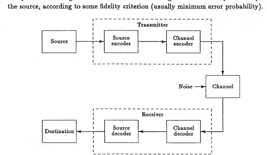
transmitter consists of source and channel encoders, and processes a signal from the source, which may be analog or digital (e.g. voice or data), into a form suitable for the channel, which may also be analog or digital. The receiver consists of source and channel decoders, and processes the signal received on the channel to generate the best possible replica of the source, according to some fidelity criterion (usually minimum error probability).

1---,

1 Transmitter 1

1 1

Source 1 _encoderSource Channel _encoder 1 1

1 1

-Noise -+ Channel

r---l

1 _Receiver 1

1 1

Destination 1 _decoderSource Channel _decoder 1

1 1

'I 1

-Figure 1.1 General digital communication system.

Two of the major contributors to the fundamentals of digital communication were Harry Nyquist and Claude Shannon. Nyquist [1928] showed that there is a fundamental lower limit on the bandwidth of the channel that can transmit pulses at a given signalling rate without mutual interference. Shannon laid the mathematical foundations for com-munication theory in 1948 with the publication of his paper: 'A Mathematical Theory of Communication' [Shannon, 1948aj 1948b]. This paper also created an entirely new field of endeavour, now known as information theory. Two of Shannon's most important theorems

are known as the source coding theorem and the channel coding theorem. A very readable account of information theory is given by Pierce [1980]. The contributions of Nyquist and Shannon are discussed in this section.

1.1.1 Channel

If a signal could be transmitted over a channel and arrive undisturbed at the receiver, then the channel would be ideal and communication theory would be simple. However, such ideal channels do not exist in practice. There are a number of disturbances that occur

on real channels and these introduce the possibility of errors when the receiver makes decisions on what was transmitted. Two of the most common disturbances are noise and intersymbol interference (lSI).

[image:21.581.78.504.127.376.2]

(22)

4 CHAPTER 1 INTRODUCTION

AWGN is not always the dominant disturbance on a channeL Another disturbance,

first experienced with early telegraph systems like Morse's (particularly with underground or undersea circuits, due to their high parallel capacitance), is that if a square pulse is

transmitted it will be received as a spread out pulse. This phenomenon is illustrated in

Figure 1.2. The speed of transmission is thus limited, because if pulses are transmitted too rapidly they will overlap in the receiver so that the receiver cannot sample one pulse without sampling part of another. Thus, the received pulses interfere with each other and decision errors result. This spreading of pulses so that they interfere with each other is known as lSI and is the predominant cause of error in many digital communication systems.

Figure 1.2 Spreading of a square pulse by the channel.

lSI occurs whenever a digital signal is passed through a linear channel with a frequency response that is not constant over the bandwidth of the signal. Furthermore, to produce a bandwidth efficient system, the bandwidth of the transmitted signal must be limited. The aim, therefore, is to design pulse shapes that occupy a minimum amount of bandwidth, and which result in a minimum of potential lSI.

Nyquist [1928] was one of the first researchers to recognize overlapping pulses as a source of interference. He is credited with formulating the criterion for zero lSI-the Nyquist criterion-which states that the lSI is zero if and only if T-spaced samples of the received pulse h(t) satisfy

h( iT)

= {

1 for

~

=

0

o

for ~ = ±1, ±2, ...

(1.1)

for a signalling rate liT and where the sampling is synchronized with the pulse. In the frequency domain, this condition becomes

1 00

HIJ (J) = -

L

H(J - j IT) = K T.

3=-00

for

If I

~ 1/2T

where K is a real constant, H(J) is the channel frequency response, and HIJ (J) is the folded or aliased channel frequency response after symbol-rate sampling. The band of frequencies

If I

~ 1/2T is known as the Nyquist or minimum bandwidth. An example of

two successive Nyquist pulses is shown in Figure 1.3a. Notice that if the receiver samples at times iT, there will be no lSI.

Assuming that a pulse has been designed to satisfy the Nyquist criterion at a signalling rate liT, lSI can be introduced by time-dispersion of the pulses in the channel or by modem imperfections (e.g. timing and carrier recovery errors, jitter, and imperfect filter design).

(23)

1.1 FUNDAMENTALS OF DIGITAL COMMUNICATION 5

4T Time

(a) Two successive Nyquist pulses

4T Time

(b) Spread Nyquist pulse

Figure 1.3 Examples of band-limited pulses.

A spread pulse is shown in Figure 1.3b. This pulse does not satisfy Nyquist's criterion for zero lSI. The main sample h(O) is called the cursor of the sampled pulse, the samples

h( iT) for i

<

0 are called precursors, and the samples h( iT) for i

>

0 are called postcursors. lSI is typically mitigated in the receiver with an equalizer that attempts to cancel the effects of lSI by performing an inverse operation to the channel. If the channel is time varying (non-stationary), the equalizer can be designed to adapt to the changing channel conditions.

Nyquist [1928] also showed that the maximum number of distinct symbols that can be sent over a channel per second is twice the total bandwidth of frequencies used. Thus, the rate that symbols can be transmitted-the signalling rate-is proportional to band-width. The dual to this theorem is the Nyquist sampling theorem, which states that an analog signal with highest frequency component W can be represented completely and reconstructed perfectly over a time T seconds from a set of 2WT samples of its amplitude

spaced 1/2W seconds apart.

1.1.2 Source Encoder and Decoder

Following the work of Nyquist, Shannon [1948a] defined a logarithmic measure of infor-mation. At the suggestion of J. W. Tukey, he called the unit of information a 'bit'-a contraction of 'binary digit'. Shannon also defined the entropy of a random source U, with specific messages u E U, as

H(U) = -

2:

P [U = u]log2 P (U =

u]

(1.3)

uEU

(24)

6 CHAPTER 1 INTRODUCTION

Suppose that the channel, channel encoder, and channel decoder form an error-free (noiseless) channel of finite capacity. Shannon's fundamental theorem for the noiseless channel [Shannon, 1948a] can be expressed as follows. Consider a noiseless channel with finite capacity C bitsls and a source with entropy H bits per symboL It is possible to encode the output of the source in such a way as to transmit at the average rate C

I

H - € symbols per second over the channel, where € is arbitrarily small. It is not possible to

transmit at an average rate greater than C

I

H. This theorem is also known as the source coding theorem.

The source coding theorem suggests the removal of redundant information from the source, using source coding, so that the encoded source rate R does not exceed the ca-pacity of the channel (R ~ C). The encoded source rate cannot be less than the rate of entropy of the source

HIT,

without losing information. Morse code is an early exam-ple of source coding, where the most common letters of the alphabet are represented by the shortest codewords. If the source encoder mapping is one-to-one, the source decoder can simply perform the inverse mapping and deliver an exact replica of the source to the destination. When the source is analog, however, it cannot be represented perfectly by a digital sequence because the amplitude samples of the analog signal take on a continuum of values. In this case some distortion must be tolerated at the destination because the source decoder can only approximate the inverse mapping.

1.1.3 Channel Encoder and Decoder

Shannon [1948a] formulated an upper bound for the rate that information could be sent, with arbitrarily low error probability, over a band-limited additive white Gaussian noise (AWGN) channeL He used a geometrical representation of the channel to prove that the bound is exact [Shannon, 1949]. The upper bound is commonly known as the channel capacity

C = _Wlog2(1

+

SIN)

(1.4)

where W is the channel bandwidth, S is the signal power, and N is the noise power. This can be rearranged to give a theoretical limit on bandwidth efficiency

(=

CIW

= log2(1

+

SIN)

(1.5)

Shannon's fundamental result for the noisy channel [Shannon, 1948a] can be expressed as follows. If the rate of entropy of the source does not exceed the capacity of a Gaussian noise channel

(HIT

~

C),

then messages from the source can be transmitted over the channel with an arbitrarily small probability of error P[£]. It is not possible to achieve an arbitrarily small probability of error if

HIT> C.

This theorem is also known as the

channel coding theorem.

The channel coding theorem implies the addition of redundancy, using a channel en-coder, to achieve arbitrarily small error probability, and as such is a dual to the source coding theorem. The goal of the channel encoder and decoder is to map the input data symbols into channel input symbols and conversely the channel output symbols into output data symbols, such that the effect of the channel noise is minimized.

(25)

1.1 FUNDAMENTALS OF DIGITAL COMMUNICATION 7

As a result of Shannon's theories we have seen the development of sophisticated channel coding techniques-as well as source coding techniques-in an effort to design bandwidth efficient systems and to approach the channel capacity.

Channel coding requires the transmission of redundant bits. These additional bits can be sent, without reducing the information rate, in one of two ways: either the sig-nalling rate can be increased, if the channel bandwidth can be expanded, or the number of channel signals can be increased, if the channel is band-limited. However, the latter tech-nique gives disappointing results when the coding and modulation operations are designed independently in the conventional manner.

Trellis-coded modulation (TCM) is a relatively new technique, developed in the 1970s by Ungerboeck [1982], that combines the functions of channel coding and modulation. The performance of a system can be improved by TCM without sacrificing data rate or requiring bandwidth expansion.

1.1.4 Design Goals and Constraints

The fundamentals of digital communication can be summarized by a list of goals and constraints that characterize the design of digital communication systems. There are a number of goals that we seek to achieve in designing a communication system:

1. Maximize the information rate R.

2. Minimize the probability of error

P[£].

3. Minimize the transmit power S.

4. Minimize the required system bandwidth W.

5. Maximize the system use.

6. Minimize the system complexity, computational load, and system cost.

Most of these goals are in conflict with each other. Shannon, however, has shown us that 1 and 2 can be achieved independently, provided R ::; C. In seeking to achieve all the above goals, the designer faces a number of theoretical and regulatory constraints:

1. Nyquist theoretical minimum bandwidth requirement.

2. Source coding theorem.

3. Channel coding theorem.

4. Regulations (e.g. spectrum allocations).

5. Technological limitations.

6. Other system requirements (e.g. satellite orbits).

(26)

8 CHAPTER 1 INTRODUCTION

1.2

Aim of the Thesis

Most long distance transmission systems use either copper circuits, optical fibre, satel-lite repeaters, or terrestrial microwave radio. In this thesis we will concentrate on digital microwave radio (DMR) systems, although the techniques and results presented are ap-plicable to other channels. DMR uses line-of-sight propagation and repeaters to transmit over long distances. The major impairment on DMR channels is sporadic multipath prop-agation. This results in multiple versions of the same signal, with different attenuation and delay, arriving at the receiver and interfering with each other. Multipath propagation is caused by inhomogeneous temperature and humidity profiles in the atmosphere. Fortu-nately, the rate.offading is slow compared to the signalling rate, and adaptive equalization can be used to reduce the severe lSI that results from deep fades.

We consider the performance of TCM on DMR systems. TCM is particularly suited to DMR systems because it can provide large coding gains without incurring a loss of bandwidth efficiency. Specifically, we study how TCM performs with residual lSI (i.e. the

lSI that remains after non-ideal equalization), since TCM cannot be expected to cope with the raw lSI generated bya severe fade. Note that residual lSI could also include lSI due

to modem imperfections, although we do not consider this situation. We wish to show that the performance of a trellis-coded system with residual lSI is superior to that of an equivalent uncoded system. This corresponds to trading code complexity for improved performance. TCM also allows code complexity to be traded for reduced transmit power or increased bandwidth efficiency.

The performance of TCM on an AWGN channel is well established in terms of lower and upper bounds on error probability and an asymptotic coding gain at high SNRs (see Section 3.4). These results extend directly to the DMR channel under normal (unfaded) propagation conditions and under fiat fading conditions. The performance of TCM with time-dispersive fading is not so well defined, and we concentrate on this problem.

In this investigation, both simulation and analytical techniques have been used. The simulation study used Monte Carlo techniques whereby the system was simulated in com-puter software, data were transmitted over the system, and the frequency of errors in the received data was monitored. Computer simulations, however, are notoriously slow and limited in practice to high bit error rates (BERs). This inevitably leads to a search for analytical solutions. The most desirable analytical solution is a tractable closed-form expression for the error probability. Unfortunately, such expressions rarely exist, and an-alytical bounds on the error probability must be used. The approach taken here is to compute a good approximation to the probability density of the lSI in the receiver and to use this in the formulation of a union bound on the error event probability in the Viterbi decoder.

(27)

Chapter

2

Some Mathematical Preliminaries

The mathematical foundations of digital communication are well established. Wozencraft and Jacobs [1965] popularized the geometric representation of signals, which is discussed in Section 2.1, although the concept was first used by Shannon [1949]. Section 2.2 showd how bandpass signals and linear bandpass systems can be represented by equivalent low-pass forms to simplify the analysis of bandlow-pass systems. Equivalent lowlow-pass signals and geometric representations are used in Section 2.3 to discuss the operation of components of bandpass systems. This chapter does not provide a complete mathematical basis for com-munication theory, but merely introduces some basic terminology used in subsequent chap-ters. There are many books that give comprehensive accounts of communication theory, for example Wozencraft and Jacobs [1965], Viterbi and Omura [1979], and Proakis [1989].

2.1

Geometric Representation of Signals

An L-dimensional orthogonal space is defined by a set of L linearly independent basis functions {c,oj(t)}. Any arbitrary function in the space can be generated by a linear combination of these basis functions, provided they satisfy the orthogonality condition

J

OO { K· if j = k

c,oj( t)c,ok( t) dt = J .

-00 0 otherWIse

forj,k=l, ... ,L (2.1)

where the constants {Kj} are nonzero. When the basis functions are normalized so each

Kj

=

1, the space is called orthonormal.

Any arbitrary set of M waveforms {yi(t)} can be expressed as a linear combination of

L (::; M) orthogonal waveforms {c,oj(t)}, such that L

Yi( t) =

I::

Yij c,oj ( t) for i = 1, . .. ,M (2.2)

j=l

where

1

Joo

Yij = K. Yi(t)c,oj(t) dt

J - 0 0

for i

=

1, ... , M and j

=

1, ... , L (2.3) The form of the basis functions {c,oj( t)} is chosen for convenience and depends on the form of the signal waveforms. The waveform Yi(t) can be viewed as a vector or signal point

(28)

10 CHAPTER 2 SOME MATHEMATICAL PRELIMINARIES

Euclidean distance is a generalization of the concept of distance in three-dimensional physical space.

The set of M signal points in the signal space is called a signal set or a signal con-stellation. Baseband signals are inherently one-dimensional and can be represented by a

scalar variable. Bandpass signals are inherently two-dimensional and can be represented by a complex variable, as discussed in the next section. Signals of higher dimensionality can be constructed using time- or frequency-orthogonal signals.

2.2

Representation of Bandpass Signals

A bandpass signal with carrier frequency fe can be represented as

yet)

=

aCt) cos(27r fet

+

OCt)) (2.4)

where aCt) is the amplitude envelope of the signal and OCt) is the phase of the signal. The

cosine can be expanded to yield

(2.5)

where the in-phase component xe(t) ~ aCt) cos OCt) and the quadrature component xs(t) ~ aCt) sinO(t) are lowpass signals. From these lowpass signals we can define a complex envelope

x(t) ~ a(t)e,7l1(t)

= xe(t)

+

JXs(t)

(2.6)

so that the bandpass signal can be represented as

(2.7)

The complex envelope defines all the characteristics of the bandpass signal, except the carrier. Since the carrier does not convey information, we can represent the bandpass signal by the equivalent lowpass signal x(t). Similarly, a linear bandpass system can be

represented by an equivalent lowpass impulse response h(t) [Proakis, 1989].

A linear bandpass system can be analyzed with complex envelopes. When a bandpass signal with complex envelope x(t) is applied to a bandpass system with complex impulse

response h(t), the complex envelope of the output can be expressed as [Proakis, 1989]

ret) =

i:

x(r)h(t - r) dr (2.8)

Complex envelopes are universally used in the analysis of bandpass systems, and are particularly useful for simulation because the carrier need not be simulated. Simulating the carrier would require a sampling rate in excess of twice the carrier frequency. A discrete Fourier transform performed using a fast Fourier transform algorithm [Oppenheim and

(29)

2.3 ANALYSIS OF BANDPASS SYSTEMS 11

2.3

Analysis of Bandpass Systems

The geometric representation of signals facilitates the use of equivalent discrete-time vec-tor systems to analyze digital communication systems. Figure 2.1 shows a discrete-time communication system where the signals are two-dimensional vectors, represented by com-plex variables. The system transmits a random message U, with specific value 'U E U, by mapping it to a signal X = feU), with specific value

:v

E X. The channel disturbs the signal to form the received signal R with specific value r from which a decision it, E U

must be made. Wozencraft and Jacobs [1965] discuss general L-dimensional systems.

Disturbance

•

1L --!Io-Transmitter :z: Channel r Receiver

r----Figure 2.1 Discrete-time communication system.

The transmitter, receiver, and performance ofthe receiver are discussed in this section.

2.3.1

Transmitter

Consider a bandpass system that transmits a single pulse

:vet)

with shape hT

(t).

The transmitted signal can be represented as

for i

=

1,2, ... , M (2.9) where

{:v

= Aic

+

JAi.,} are M possible complex pulse amplitudes. If the pulse shape

hT

(t)

is square and its duration is a multiple of the carrier period 1/ fc (or much greater

than it), then basis functions for the signal space are CPl(t)

=

hT (t) cos(27r'fct) and

CP2(t) = hT (t) sin(27r fet ) , and {(Aic, Ais)} are points in a two-dimensional signal space. The bandpass transmitter can thus be represented as in Figure 2.2, where the signal mapper is the equivalent lowpass transmitter.

1L

Signal mapper

1(,)

Impulse generator

Figure 2.2 Bandpass transmitter.

Yi(t)

When Ai.,

=

0 for i

=

1,2, ... , M, the signal points only occupy one dimension of the signal space, and the bandpass signal is called M-ary pulse amplitude modulation

(M-PAM). A 4-PAM signal constellation is illustrated in Figure 2.3a.

Bandpass PAM signals use bandwidth inefficiently unless single sideband transmission

is used [Proakis, 1989, Chapter 3]. This involves removing the redundant sideband, and requires expensive hardware. A more efficient bandpass signal is obtained when the M

signal points {(Aic, Ai.,)} form a rectangular grid, as shown in Figure 2.3b for M = 16. This modulation is called M-ary quadrature amplitude modulation (M-QAM).

When a system is severely nonlinear (e.g. when the high power amplifier is in

(30)

12 CHAPTER 2 SOME MATHEMATICAL PRELIMINARIES

The problem of amplitude distortion can be avoided by using M-ary phase-shift key-ing (M-PSK), which transmits information using only the phase of the carrier. This can be achieved by using signal points with constant amplitude

J

Atc

+

Ars'

and phase tan-1

(Ais/Aic)

₌_{27ri/M. An 8-PSK signal constellation is shown in Figure 2.3c.}

!P2 (t) !P2( t) !P2( t)

4& 4& 4&

..

•

!Pl (t)

..

•

..

!Pl (t)

•

!Pl (t)

•

• •

•

4& 4& 4&

•

(a) 4-PAM (b) 16-QAM (c) 8-PSK

Figure 2.3 Examples of signal constellations.

If a sequence of symbols (pulses) is transmitted, the equivalent lowpass signal trans-mitted over the channel is

00

(2.10)

n=-oo

where {xn} is the sequence of complex symbols and hT

(t)

should satisfy the Nyquist criterion for zero lSI when sampled at t

=

nT for integer n. The condition for zero lSI

is essentially a time-orthogonality condition. Time-orthogonal pulses can be used to form signals with more than two dimensions. In an analogous manner, frequency-orthogonal signals can be used to add further dimensions.

2.3.2 Receiver

The most appropriate-but generally intractable-criterion for designing an optimum re-ceiver is to minimize the probability of an erroneous symbol decision

pre],

or equivalently to maximize the probability of a correct decision

P[C]

=

i:

P

[C

I

R

=

r ] PR (r) dr (2.11) where P [C

I

R

=

r] is the probability of a correct decision conditioned on R, and P R (r) is the probability density function (pdf) of R. From (2.11) we see that P[C] is maximized when

P [C

I

R =

r]

is maximized. When the receiver sets

u

=

u',

the conditional probability of a correct decision is

P

[C

I

R

=

r]

=

P [

u

=

u'

I

R

=

r]

(2.12)

where P [U

=

u'

I

R

=

r] is the a posteriori probability of message u' having been trans-mitted.

To avoid cumbersome notation in subsequent chapters, we use the equivalent notation

P

[a]

==

P [A =

a]

for all a E

A

(2.13)

where A is usually a discrete random variable with specific value a E

A.

We also use

(31)

2.3 ANALYSIS OF BANDPASS SYSTEMS 13

where B is usually a continuous random variable with specific value b. This notation will

be used when there is no possibility of ambiguity.

The optimum receiver must determine, for a given received signal, which of the mes-sages u E U has maximum a posteriori probability (MAP). The so called MAP receiver uses its knowledge of the conditional pdf P ( r

I

x), the signal set X, and the a priori

message probabilities p

[u]

to set it,

=

u'

whenever

p [ u'

I

r]

>

P [ u

I

r ] for all u f=. u' and u, u' E U (2.15) If two or more messages have MAP, the receiver arbitrarily selects one of them. Using the mixed form of Bayes' rule [Wozencraft and Jacobs, 1965, Chapter 2]

p

[u'

I

r]

=

P[u']:(~)

I

u')

(2.16) and

P (

r

I

u')

=

P

(r

I

x')

for u' E U and x'

=

feu') E X (2.17) where

fO

is the signal mapping function. Since P (r) is independent of the transmitted message, the MAP receiver sets it, = u' whenever the decision function

p

[u']

P.(

rl

x')

for u' E U and x' = feu') EX (2.18)

.

IS maxImum.

The a priori message probabilities p

[u]

are often unknown. In such cases, the receiver can determine it, to maximize p( r

I

x). This receiver is called a maximum-likelihood (ML)

receiver, and is optimum when all messages are equally likely.

If the disturbance on the channel is additive white Gaussian noise (AWGN), the re-ceived signal is r

=

x

+

'f}, where 'f} is a specific value of a complex Gaussian random variable

N.

The AWGN actually has an infinite number of dimensions, but only the vec-tors that lie within the signal space are relevant to the decision process [Wozencraft and Jacobs, 1965, Chapter 4]. The ML receiver determines it, by maximizing

P ( r

I

x')

=

PN ( r - x'

I

x') (2.19)

The random variables

N

and X are usually statistically independent, so

PN ( r - x'

I

x')

=

PN (r - x') for all x' E X (2.20) The pdf of the Gaussian noise is

1

(10:

12 )

PN(O:) = exp -27ra2 _2a2

'1 '1

(2.21)

with zero mean and variance a~. Therefore, maximizing P ( r

I

x') = PN (r - x') is equiv-alent to minimizing

Ir - x'1

2• Geometrically,

Ir - x'1

2 is the squared Euclidean distance between points r and x' in the signal space. Thus the ML decision rule assigns the re-ceived point r to u' if and only if r is closer to x' =

f(

u~) than any other signal point. This decision rule can be used to partition the signal space into M disjoint regions {Au}

so that whenever the received vector r is in Aul the receiver sets it, = u'

(32)

14 CHAPTER 2 SOME MATHEMATICAL PRELIMINARIES

... _...

•

,

"

_... _.-, , V'1 (t)

"

,

.-•

[image:32.572.258.380.60.168.2]

•

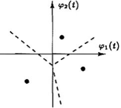
Figure 2.4 ML decision regions for three signal points.

These regions are called decision regions and are illustrated in Figure 2.4 for three equally likely signal points. For the ML decision rule, the decision boundary between any two signal points is the perpendicular bisector of a line between the points.

Before the receiver can apply a decision rule, it must extract a received signal vector from the received signal. In the absence of noise, the receiver can extract the received signal vector from ret) by correlating ret) with each of the basis functions tpj(t), as implied by

(2.3); this forms the basis of the correlation receiver shown in Figure 2.5a. When noise

is present, the correlation receiver maximizes the signal-to-noise ratio [Wozencraft and

Jacobs, 1965, Chapter 4]. The correlators in the correlation receiver can equivalently be implemented by matched filters {tpj(T - tn sampled at time T, to obtain the matched filter receiver shown in Figure 2.5b. The basis functions {tpj(tn should be zero for t

>

T

T(t)

V'l(t)

(a) Correlation receiver

(b) Matched filter receiver

Decision rule

Figure 2.5 ML bandpass receivers.

[image:32.572.164.459.378.656.2]

(33)

2.3 ANALYSIS OF BANDPASS SYSTEMS 15

correlation operations.

A system that transmits a square pulse hT

(t)

requires an infinite bandwidth channel to avoid distortion, but in practice we are usually interested in limited or near band-limited (most of the pulse energy within a finite bandwidth) systems. Also, a system that transmits a single message is not very useful; therefore, we are usually interested in systems that can transmit sequences of messages. Both these issues can be addressed by designing band-limited pulses that satisfy Nyquist's criterion for zero lSI (time-orthogonality). Se-quences of messages can be transmitted and received by time-sharing the transmitter and receiver over successive messages.

H

the Nyquist pulses are distorted on the channel, the pulses are no longer time-orthogonal and lSI results in the receiver.

When a channel introduces lSI in addition to AWGN, the linear receivers just described are no longer optimum. The optimum linear receiver becomes a sampled matched filter followed by an inverse filter (infinite-tap transversal equalizer) prior to applying the ML decision rule [Proakis, 1989, Chapter 6]. This receiver will enhance the Gaussian noise and is not globally optimum. An optimum nonlinear receiver that does not enhance the Gaussian noise is described by Forney [1972]. This receiver consists of a whitened matched

filter followed by ma:cimum-likelihood sequence estimation. The whitened matched filter

consists of a matched filter followed by a transversal filter to whiten the noise. The noise must be whitened so that a squared Euclidean distance metric can be used with the Viterbi algorithm, to determine the maximum-likelihood transmitted sequence. The difficulty of implementing Forney's receiver has prompted a number of researchers to examine suboptimum, but realizable, receivers for lSI channels [Magee and Proakis, 1973; Qureshi and Newhall, 1973; Falconer and Magee, 1973; Ungerboeck, 1974; Eyuboglu and Qureshi, 1988].

2.3.3 Performance of the Receiver

The decision error probability

Pre]

forms the basis of most performance measures. In practice, bit error rate (BER) or symbol error rate (SER) are usedj these measures are defined as the ratio of the number of errored data units to total data units over a specified time interval.

The probability of a symbol decision error can be expressed as

P.[E] =

L

p[u]P.[E 11£] (2.23)

uEU

Defining {Au} as the set of erroneous decision regions for messages '1.1. E U, the conditional probability of a symbol decision error is

For an AWGN channel

P"

[e

I

'1.1.] = P [ r E

Au

I

'1.1.]

=

f

p( r 1

/('1.1.»

dr

h.. ..

(2.24)

(2.25)

(2.26)

(2.27)

(34)

16 CHAPTER 2 SOME MATHEMATICAL PRELIMINARIES

The decision regions for an ML receiver are illustrated in Figure 2.6 for M = 8. The two points

±(M - 1)d/2

have a conditional symbol error probability of

(2.28)

where

fOO 2

Q

(s)

=

is

e-

t /2 dt (2.29)

is the Gaussian integral function, also referred to as the Q-function. The other M - 2 signal points have

(2.30)

Using (2.23) with P

[u]

= 11M we get an expression for the probability of a symbol error

(2.31)

I I

I I I I

I _I I I _I I

I

I - 3 d ~ -2d I

I - d 0 I Id ~2d I 13d

Figure 2.6 ML decision regions for M-PAM.

It is often not possible to form a tractable analytical expression for the decision error probability of a system, especially when the system uses channel coding or the channel introduces lSI. In these cases it is necessary to use probability bounds to estimate the probability of an error. In Chapter 7 we will use the Union, Chernoff, and Viterbi bounds that are introduced below.

Union Bound

Expressions for p[e] usually involve the probability of a union of events

P

[U~l

Ai],

where

{Ad is a set of events from the set

n.

This union is difficult to evaluate exactly, especially for large K. An examination of the Venn diagram in Figure 2.7 shows that, for K = 3,

(2.32)

This is true for any K, and the bound is known as the union bound [Wozencraft and

(35)

2.3 ANALYSIS OF BANDPASS SYSTEMS

Chernoff Bound

I

,

~ ~

,

"" ...

--

....

I

A1 U A2 U A3

'> __

I

..

---+-=.-=--I

I I

I

,

"

~

..

Figure 2.7 Venn diagram for K = 3 intersecting events.

The Chernoff bound for a single random variable Y is derived by Proakis [1989] as

>.,

€

2::

0

where E [.] is the expected value and the Chernoff parameter>' is determined from

:>.

E [eA(Y-€)]

=

0

Viterbi Bound

A bound that generally yields tighter bounds than the Chernoff bound is given by

U, 'U

2::

0 _

17

(2.33)

(2.34)

(2.35)

We call this bound the Viterbi bound because Viterbi [1971] appears to be the first re-searcher to have applied it to digital communication problems~ It can be proven by writing the Q-functions in terms of integrals. The right-hand side of (2.35) gives

e-v/ 2

Q (02)

= e-v/ 2_ _ ₁

1

00 e-s ₂_/2_ds

..;2i..;u

= _1_

1

00 e-(v+s2)/2 ds

..;2i..;u

(2.36)

Using the substitution 'U

+

s2 = w2 and hence ds = wdwjJw2 - 'U, we get

e-v/ 2

Q (02)

= _1_

1

00

w e-w2 /2 _dw

..;2i

v'U+u

J

w2 _- _'U (2.37)

Since 'U

2::

0, it follows that w

2::

0 and w j Jw2 - 'U

2::

1. Using these inequalities, we can write the inequality

_1_

1

00 e-t2/2 dt

<

_1_

1

00 w e-w2 / 2 dw

..;2i

.ju+v

-..;2i

.ju+v J w 2 - 'U

::; e-v/2 Q

(v'u)

(2.38)

(36)

18 CHAPTER 2 SOME MATHEMATICAL PRELIMINARIES

2.4

Conclusion

(37)

Chapter

3

Trellis-Coded Modulation

In a conventional data transmission system, the channel encoder and signal mapping func-tion of the modulator are de~igned independently, so that the channel coding is essentially an addition to an un coded system. The code redundancy is accommodated by reducing the data rate or by increasing the system bandwidth. In either case, the bandwidth efficiency is reduced relative to the uncoded system. The modulator maps m-bit code symbols into one of 2~ possible channel symbols. Gray encoding is usually used so that neighbouring

signal points in the constellation are assigned to code symbols that diff'er in only one bit. Hence, the most likely symbol decision errors only result in single bit errors, and the bit error probability is minimized. The demodulator uses the maximum-likelihood decision rule to make a hard decision on the m-bit code symbol, and the decoder then determines

the source symbol from the code symbol. If the code symbols are binary words, Ham-ming distance is the metric used for decoding, and the code is designed to maximize the minimum Hamming distance.

The concept of coded modulation is to accommodate the· code redundancy by expanding

the signal constellation so that the bandwidth efficiency of the system relative to the uncoded system is unchanged. The channel encoder and signal mapping function of the modulator are designed jointly to maximize the free distance (djree) of the code. In the

receiver, the decoding and detection operations are also combined so that the decoder operates on soft decisions, using the metric for which the code was designed. Section 3.1

illustrates how coded modulation can be used to approach Shannon's capacity bound, and some trade-off's that can be achieved.

Coded modulation was invented in the 1970s by Ungerboeck [1982]' who developed schemes, which are known as trellis-coded modulation (TCM), based on convolutional codes. The TCM schemes described by Ungerboeck are optimized for additive white Gaussian noise (AWGN) channels and will be referred to as Ungerboeck codes. Ungerboeck

encoding involves the convolutional encoding of source symbols followed by the mapping of coded symbols onto an expanded signal set, using a technique called mapping by set partitioning to maxi~ze the free Euclidean distance of the code. This process can be represented as a trellis of states with restricted paths, and is described in Section 3.2 with an illustrative example.

The optimum receiver for an Ungerboeck code on an AWGN channel performs soft-decision maximum-likelihood sequence estimation, usually using the Viterbi algorithm.

(38)

20 CHAPTER 3 TRELLIS-CODED MODULATION

non-AWGN disturbances. The time-dispersive channels investigated in this thesis are of this type. Nevertheless, in the absence of a better metric, the squared Euclidean distance metric is retained.

Coding gain is a measure of the performance of a coded system relative to an un-coded system. TCM can achieve significant coding gains on AWGN channels, relative to

uncoded systems, without sacrificing data rate or requiring bandwidth expansion. For ex-ample, simple 4-state TCM schemes can achieve a 3 dB asymptotic coding gain, while more

sophisticated TCM schemes have asymptotic coding gains of up to 6 dB. The performance of TCM, decoded using soft-decision Viterbi decoding, is discussed in Section 3.4

We will only study Ungerboeck codes in detail; however, it should be noted that there are other coded modulations that can achieve the same, or higher, coding gains with less complexity. To achieve asymptotic coding gains of 6 dB without using impractical codes, TCM schemes can be designed with multidimensional signal constellations to spread the constellation expansion over more than one signalling interval [Ungerboeck, 1987aj Wei, 1987]. Another variation on Ungerboeck codes is the rotationally invariant codes designed by Wei [1984aj 1984b].

Calderbank and Sloane [1987] have formulated a general class of coded modulations known as coset codes, which includes Ungerboeck codes. The signal constellation is

re-garded as a finite subset of points from an infinite lattice, and set partitioning of the constellation is regarded as a partitioning of the lattice into a sublattice and its cosets. The theory of coset codes has been refined by Forney [1988aj 1988b]. Ungerboeck codes represent some of the best codes in the class of known coset codes. Multilevel codes are a

generalization of coset codes that can achieve the coding gains of single level coset codes, with reduced complexity decoding [Calderbank, 1989; Pottie and Taylor, 1989a].

3.1

Approaching Shannon's Bound

A natural question to consider is: how closely can coded modulation systems theoretically operate to Shannon's bound? This issue was addressed by Ungerboeck [1982]. Shannon's capacity bound for an AWGN channel is expressed as a bandwidth efficiency bound in (1.5). When a signal constellation is specified and soft-decision decoding is used, Unger-boeck [1982] has shown how to compute the maximum bandwidth efficiency when the signal constellation is used on an AWGN channel. The bandwidth efficiency bound is plotted as a function of signal-to-noise ratio (SNR) in Figure 3.1, together with the maxi-mum bandwidth efficiencies of several signal constellations [Ungerboeck, 1982]. Note that the maximum bandwidth efficiency of the constellations is always less than Shannon's bound.

(39)

3.1 APPROACHING SHANNON'S BOUND

;a

---

III

---

....

III

4

e

3

4-PSK

Il.

uncoded P.[t:] = 10-6

o

coded p.[t:] = 10-6

5 10 15 20

Signal-to-noise ratio (dB)

[image:39.582.69.513.60.356.2]

25

Figure 3.1 Bandwidth efficiency versus signal-to-noise ratio curves.

modulation.

21

While actual coded modulation schemes have been designed that operate close to the Shannon bound, the cut-off rate Ro is regarded by many researchers as a limit to the capacity that can be readily achieved in practice [Forney et al., 1984]. The complexity of sequential decoders is also known to grow rapidly as the code rate is increased above Ro

[Wozencraft and Jacobs, 1965]. A detailed discussion of Ro is provided by Wozencraft and Jacobs [1965]. For an AWGN channel

Ro = Wlog2(1

+

S/2N) (3.1)

so Ro is always less than the channel capacity for a given S / N

>

O. Coded modulations can be designed with asymptotic coding gains of 6 dB; these codes achieve Ro •

lf we plot points of equal symbol error probability for the uncoded constellations and typical coded constellations on