The Design of Output Feedback Distributed Model Predictive Controller for a Class of Nonlinear Systems

ISSN Online: 2152-7393 ISSN Print: 2152-7385

DOI: 10.4236/am.2017.812131 Dec. 29, 2017 1832 Applied Mathematics

The Design of Output Feedback Distributed

Model Predictive Controller for a Class of

Nonlinear Systems

Baili Su, Yingzhi Wang

College of Engineering, Qufu Normal University, Rizhao, China

Abstract

For a class of nonlinear systems whose states are immeasurable, when the outputs of the system are sampled asynchronously, by introducing a state ob-server, an output feedback distributed model predictive control algorithm is proposed. It is proved that the errors of estimated states and the actual sys-tem's states are bounded. And it is guaranteed that the estimated states of the closed-loop system are ultimately bounded in a region containing the origin. As a result, the states of the actual system are ultimately bounded. A simula-tion example verifies the effectiveness of the proposed distributed control method.

Keywords

Nonlinear Systems, Distributed Model Predictive Control, State Observer, Output Feedback, Asynchronous Measurements

1. Introduction

Traditional process control systems just simply combine the measurement sen-sors with control actuators to ensure the stability of closed-loop systems. Al-though this paradigm to process control has been successful, the calculation burden of this kind of control is large and the performance of the system is not good enough [1]. So far the stability of closed-loop systems has been guaranteed and at the same time, the performance of the closed-loop systems has been im-proved if the control systems are divided into local control systems (LCS) and networked control systems (NCS). And it can reduce the burden of calculation. But this kind of transformation needs to redesign LCS and NCS to ensure the stability of closed-loop systems. As a result, the control strategy is changed [2].

How to cite this paper: Su, B.L. and Wang, Y.Z. (2017) The Design of Output Feedback Distributed Model Predictive Controller for a Class of Nonlinear Systems. Applied Mathematics, 8, 1832-1850.

https://doi.org/10.4236/am.2017.812131 Received: December 1, 2017

Accepted: December 26, 2017 Published: December 29, 2017

Copyright © 2017 by authors and Scientific Research Publishing Inc. This work is licensed under the Creative Commons Attribution International License (CC BY 4.0).

http://creativecommons.org/licenses/by/4.0/

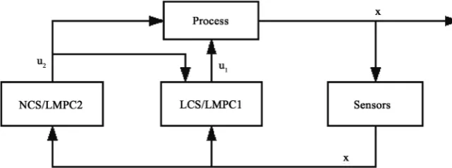
DOI: 10.4236/am.2017.812131 1833 Applied Mathematics Model predictive control (MPC) is receding horizon control which can deal with the constraints of systems’ inputs and states during the design of optimiza-tion control. It adopts feedback correcoptimiza-tion, rolling optimizaoptimiza-tion, and has strong ability to deal with constraints and dynamic performance [3] [4] [5]. Therefore, it can be more effective to solve the optimal control problem for distributed sys-tems. That is distributed model predictive control [6]. The distributed model predictive control takes into account the actions of the local controller in the calculation of its optimal input trajectories. At the same time, LCS and NCS are designed via Lyapunov-based model predictive control (LMPC). But when the LCS is a model predictive control system for which there is no explicit control formula to complete its future control actions, it is necessary to redesign both the NCS and LCS and establish some communication between them so that they can coordinate their actions. We refer to the trajectories of u1 and u2 as LMPC1 and LMPC2. The structure of the system is as Figure 1.

There are many research results about distributed MPC design at present. In literature [7], a novel partition method of distributed model predictive control for a class of large-scale systems is presented. Literature [8] presents a coopera-tive distributed model prediccoopera-tive control algorithm for a team of linear subsys-tems with the coupled cost and coupled constraints. A distributed model predic-tive control architecture of nonlinear systems is studied in literature [2]. Based on literature [2], literature [9] considers a distributed model predictive control method subject to asynchronous and delayed measurements. A distributed model predictive control strategy for interconnected process systems is proposed in reference [10]. In literature [11], a design approach of robust distributed model predictive control is proposed for polytopic uncertain networked control systems with time delays. Reference [12] presents that the distributed model predictive control method is applied for an accurate model of an irrigation canal. For a hybrid system that comprises wind and photovoltaic generation subsys-tems, a battery bank and an ac load, a distributed model predictive control me-thod is designed to ensure the closed-loop system stable in reference [13].

[image:2.595.210.531.586.705.2]

These references are obtained on the assumption that the systems’ states can be measured continuously. The systems whose states are immeasurable are not taken into account in these references. However, immeasurable states often

DOI: 10.4236/am.2017.812131 1834 Applied Mathematics happen in practice. In literature [14], under the condition that the states are not measured, a distributed model predictive control algorithm for interconnected systems based on neighbor-to-neighbor communication is presented. Literature

[15] considers the design of robust output feedback distributed model predictive control when the dynamics and measurements of systems are affected by bounded noise. But both literatures are studied for the linear systems. An out-put-feedback approach for nonlinear model predictive control with moving ho-rizon state estimation is proposed in reference [16]. Reference [17] considers output feedback model predictive control of stochastic nonlinear systems. Yet these two references are centralized model predictive control methods. The computational complexity grows significantly.

On the basis of the above references, this paper considers a class of nonlinear systems whose states are immeasurable. By introducing a state observer, and us-ing output feedback, under the assumption that the outputs of the system are sampled of asynchronous measurements, an output feedback distributed model predictive control algorithm is designed. Therefore, the ultimately boundedness of the estimated states and the boundedness of the error between estimated states and the actual system’s states are proved, and then it is proved that the states of the actual system are ultimately bounded. And the stability of the closed-loop system is guaranteed. The performance of the system is improved and the burden of calculation is reduced.

This paper is arranged as follows. The second section is the preparation work. In the third section, the state observer is designed, and its stability is analyzed. The fourth section designs a controller based on Lyapunov function to make sure the asymptotic stability of the nominal observer. In the fifth section, an output feedback distributed model predictive control algorithm is proposed and the stability of the closed-loop system is proved. The instance simulation is pro-vided in the sixth section. Conclusion is given in Section 7.

2. Preliminaries

2.1. Definitions and Lemmas

In this paper, the operator ⋅ denotes Euclidean norm of variates. The symbol

( )

x t denotes the derivative of x t

( )

. The symbol Ωr denotes the set

( )

{

nx :

}

r x R V x r

Ω = ∈ ≤ _{where V is a scalar positive definite, continuous}

diffe-rentiable function and V

( )

0 =0 and r is a positive constant. Definitions and

lemmas used in this paper are as follows:

Definition 1 [18]: A function f x

( )

is said to be locally Lipschitz if there

ex-ists a constant Lx such that f x

( )

1 − f x

( )

2 ≤L xx 1−x2 for all x1 and x2 in a given region of x and Lx is the associated Lipschitz constant.

Definition 2 [18]: A continuous function

γ

: 0,

[

a

)

→

[

0,∞

)

belongs to class

 if it is strictly increasing and

γ

( )

0 = 0. A continuous function β

( )

r s, is

said to belong to class  if, for fixed s, β

( )

r s, belongs to class  with

DOI: 10.4236/am.2017.812131 1835 Applied Mathematics

( )

r s, 0

β

→ as s→0. Lemma 1 [18]: Let

[

]

T

0,, 0 be an equilibrium point for the nonlinear sys-tem x= f t x

( )

, where _f : 0,

[

_{∞ × →}

)

_{D R}n is continuous differentiable,

{

n

}

D= x∈R x <r where r is a positive constant and the Jacobian matrix

[

∂ ∂f x

]

is bounded on D, uniformly in t. Let

β

be a class  function and

0

r be a positive constant such that β

(

r0, 0

)

<r. Let 0

{

0

}

n

D = x∈R x <r .

As-sume that the trajectory of the system satisfies

( )

(

( )

0 , 0

)

,

( )

0 0, 0 0

x t ≤β x t t−t ∀x t ∈D ∀ ≥ ≥t t (1)

Then, there is a continuously differentiable function V: 0,

[

∞ ×

)

D0→R that satisfies the inequalities

( )

( )

( )

( )

( )

( )

1 2

3

4

,

,

x V t x x

V V

f t x x

t x

V

x x

α α

α α

≤ ≤

∂ ∂

+ ≤ −

∂ ∂

∂ ≤ ∂

(2)

where α α α1, 2, 3 and α4 are class  functions defined on

[ ]

0,r0 . If the sys-tem is autonomous, V can be chosen independent of t.

Lemma 2 [18]: Let

[

]

T

0,, 0 be an equilibrium point for the nonlinear sys-tem x= f t x

( )

, . The equilibrium point is uniformly asymptotically stable if and only if there exist a class  function

β

and a positive constant c, indepen-dent of t0, such that

( )

(

( )

0 , 0

)

, 0 0,

( )

0

x t ≤β x t t−t ∀ ≥ ≥ ∀t t x t <c (3)

2.2. Problem Formulation

Consider a class of nonlinear systems described as follows:

( )

(

( ) ( ) ( ) ( )

)

( )

( ) ( )

1 2

, , ,

x t f x t u t u t w t y t h x υ t

=

= +



(4)

where _{x t}

( )

∈_Rnx denotes the state vector which is immeasurable.

( )

1 1

u

n

u t ∈R ,

( )

2

2

u

n

u t ∈R are control inputs. u1 and u2 are restricted to be in two non-empty convex sets 1 2

1 , 2

u u

n n

U ⊆R U ⊆R . _{w t}

( )

∈_Rnw denotes the disturbance

vector.

( )

ny

y t ∈R is the measured output and _{v t}

( )

∈_Rnv is a measurement

noise vector. The disturbance vector and noise vector are bounded such as

w∈, v∈ where

{

}

{

}

1 1

2 2

: , 0

: , 0

w

v

n

n

w R w c c

v R v c c

= ∈ ≤ >

= ∈ ≤ >



 (5)

DOI: 10.4236/am.2017.812131 1836 Applied Mathematics of system (4), y, is sampled asynchronously and measured time is denoted by

{

t_k≥0

}

such that tk = + ∆ =t₀ k ,k 0,1, with t0 being the initial time,

∆

being a fixed time interval. Generally, there exists a possibility of arbitrarily large periods of time in which the output cannot be measured, then the stability prop-erties of the system is not guaranteed. In order to study the stability propprop-erties in a deterministic framework, we assume that there exists an upper bound Tm

on the interval between two successive measured outputs such that

{

1

}

max t_k+ −t_k ≤T_m. This assumption is reasonable from a process control pers-pective.

Remark 1: Generally, distributed control systems are formulated on account of the controlled systems being decoupled or partially decoupled. However, we consider a seriously coupled process model with two sets of control inputs. This is a common phenomenon in process control.

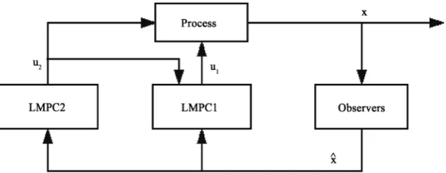
The objective of this paper is to propose an output feedback control architec-ture using a state observer when the states are immeasurable. The state observer has the potential to maintain the closed-loop stability and improve the closed-loop performance. We design two LMPCs to compute u1 and u2. The structure of the system is as follows:

Remark 2: The procedure of the system shown in Figure 2 is as follows 1) When the states are immeasurable, the observer is used to estimate the current state x.

2) LMPC2 computes the optimal input trajectory of u2 based on the esti-mated state xˆ and sends the optimal input trajectory to process and LMPC1.

3) Once LMPC1 receives the optimal input trajectory of u2, it evaluates the optimal input trajectory of u1 based on xˆ and the optimal input trajectory of

2

u .

4) LMPC1 sends the optimal input trajectory to process. 5) At next time, return step (1).

3. Observers and Property

3.1. The Design of Observers

[image:5.595.213.538.579.705.2]

Define the nominal system of system (4) as following:

DOI: 10.4236/am.2017.812131 1837 Applied Mathematics

( )

(

( ) ( ) ( )

)

( )

( )

* *

1 2

* *

, , , 0

x t f x t u t u t

y t h x

=

= 

(6)

where _x*∈_Rnx denotes the state vector of nominal systems, * ny

y ∈R is the noise free output.

Assume that there exists a deterministic nonlinear observer for the nominal system (6):

( ) ( ) ( ) ( )

(

)

* * *

1 2

ˆ ˆ , , ,

x =F x t u t u t y t (7)

such that * ˆ

x asymptotically converges x* for all the states _{x x}*,ˆ*∈_Rnx, where

* ˆ nx

x ∈R indicates the state vector of nominal observer. From Lemma 2, there

exists a class  function

β

such that:

( )

( )

(

( )

( )

)

* * * *

0 0 0

ˆ ˆ ,

x t −x t ≤β x t −x t t−t (8)

We assume that F is a locally Lipschitz vector function. Note that the conver-gence property of observer (7) is obtained based on nominal system (6) with continuous measured output.

From the Lipschitz property of f and Definition 1, there exists a positive con-stant M1 such that:

(

*

)

1 2 1

, , , 0

f x u u ≤M (9)

for all _x*∈_Rnx.

The actual observer of the system is obtained when the deterministic observer is applied to system (4). The observer of system (4) is described as follows with the state disturbance and measurement noise:

( ) ( ) ( ) ( )

(

1 2

)

ˆ ˆ , , , _k

x=F x t u t u t y t (10)

where y t

( )

k is the actual sampled measurement at tk, for ∀ ≥t tk.

3.2. The Property of Observers

In this subsection, the error between the actual system's states and estimated states will be studied under the condition of state disturbance and measurement noise when observer (10) is applied to system (4).

Theorem 1: Consider observer (10) with output measurement y t

( )

k starting from the initial condition x tˆ

( )

_k , the error of estimated state x tˆ

( )

and actual

state x t

( )

is bounded:

( )

( ) ( )

ˆ

(

( )

k , k

)

1

(

k

)

2

(

k

)

e t = x t −x t ≤β e t t−t +δ t−t +δ t−t (11)

for ∀ ≥t tk where e t

( )

k =x t

( ) ( )

k −x tˆ k is the initial error of the states, and

( )

(

)

( )

(

)

(

)

1

1 2 1

1

1

2

2 1 2

1

e 1

e 1

l

q

l c l q

bM N c

q τ

τ

δ τ

δ τ

= −

= ∆ + − (12)

DOI: 10.4236/am.2017.812131 1838 Applied Mathematics and h, respectively, and N is the predictive horizon.

Proof: For ∀ ≥t tk, from (8) and

( )

( ) ( )

( )

* *

ˆ k ˆ k , k k

x t =x t x t =x t , it can be ob-tained that:

( )

( )

(

( )

( )

)

( ) ( )

(

)

( )

(

)

* * * *

ˆ ˆ ,

ˆ , ,

k k k

k k k

k k

x t x t x t x t t t

x t x t t t

e t t t β β β − ≤ − − = − − = − (13)

Based on the Lipschitz property of f and Definition 1, there exist constants 1, 2

l l , such that:

( )

( )

(

( ) ( ) ( ) ( )

)

(

( ) ( ) ( )

)

( )

( )

( )

* *

1 2 1 2

*

1 2

, , , , , , 0

x t x t f x t u t u t w t f x t u t u t

l x t x t l w t

− = −

≤ − +

 

(14)

Because of *

( )

( )

k k

x t =x t (that is to say x*

( ) ( )

tk −x tk =0), and w t

( )

≤c1, the following inequality can be got by integrating the above inequality from tk

to

t

:

( )

*

( )

2 1

(

1( )

)

(

)

1 1

el t tk 1

k l c

x t x t t t

l δ

−

− ≤ − = − ₍₁₅₎

From the triangle inequality and inequalities (13), (15), it can be written as:

( )

( )

( )

( )

( )

( )

( )

(

)

(

)

* * * * 1 ˆ ˆ , ,

k k k k

x t x t x t x t x t x t

e t t t t t t t

β δ

− ≤ − + −

≤ − + − ∀ ≥ (16) From the Lipschitz property of F and Definition 1, there exist constants q q1, 2 satisfying the following inequality:

( ) ( )

(

( ) ( ) ( ) ( )

)

(

( ) ( ) ( ) ( )

)

( ) ( )

( ) ( )

* * *

1 2 1 2

* *

1 2

ˆ ˆ ˆ , , , ˆ , , ,

ˆ ˆ

k

k

x t x t F x t u t u t y t F x t u t u t y t

q x t x t q y t y t

− = −

≤ − + −

 

(17)

for ∀ ≥t tk. Note that

( )

(

( )

)

( )

(

( )

)

( )

* *

, _{k k k}

y t =h x t y t =h x t +

υ

t , hence:

( ) ( )

(

( )

)

(

( )

)

( )

* *

k k k

y t −y t ≤ h x t −h x t +υ t (18)

Due to the Lipschitz property of h and Definition 1, there exists a constant b such that:

( ) ( )

( ) ( )

( )

* *

k k k

y t −y t ≤b x t −x t +

υ

t (19)

Because of *

( )

( )

k k

x t =x t and the boundedness of υ, we can get:

( ) ( )

( )

( )

* * *

2

k k

y t −y t ≤b x t −x t +c (20)

From (9) and the dynamics of *

x , it can be derived that:

( )

( )

(

)

* *

1

k k

x t −x t ≤M t−t (21)

From (20) and (21), we can get:

( ) ( )

(

)

*

1 2

k k

y t −y t ≤bM t−t +c (22)

DOI: 10.4236/am.2017.812131 1839 Applied Mathematics

( ) ( )

( ) ( )

* *

1 2 1 2 2

ˆ ˆ ˆ ˆ , k

x t −x t ≤q x t −x t +q bM N∆ +q c ∀ ≥t t (23)

Integrating the above inequality from tk to

t

and taking into account of

( )

( )

*

ˆ _k ˆ _k

x t =x t , the following inequality can be got:

( ) ( )

(

)

(

1( )

)

(

)

* 2

1 2 2

1

ˆ ˆ eq t tk 1

k q

x t x t bM N c t t

q δ

−

− ≤ ∆ + − = − ₍₂₄₎

As a result, based on the triangle inequality and the inequalities (16) and (24), it can be written that:

( )

( )

( )

( ) ( )

( )

(

)

(

)

(

)

* *

1 2

ˆ ˆ ˆ

,

k k k k

e t x t x t x t x t

e t t t t t t t

β δ δ

≤ − + −

≤ − + − + − (25) That finishes the proof of the theorem.

Theorem 1 indicates that, the upper bound of the estimated error depends on several factors including initial error of the states e t

( )

k , Lipschitz properties of the system and observer dynamics, sampling time of measurements

∆

and the predictive horizon N, the bounds c1 and c2 of magnitudes of disturbances and noise, as well as open-loop operation time of the observer t−tk.

Remark 3: Because the bound of e t

( )

is the function of the observer's

open-loop operation time and the observer’s open-loop operation time is finite, the function can be restricted to a region. We assume the region is Ωe. It can be

derived that e t

( )

∈Ωe.

4. Lyapunov-Based Controller

We assume that there exists a Lyapunov-based controller u t1

( )

=g x t

( )

ˆ

( )

which satisfies the input constraints on u1 for all xˆ inside a given stability re-gion. And the origin of the nominal observer is asymptotically stable with

2 0

u = . From Lemma 1, this assumption indicates that there exist class 

functions αi

( )

⋅ and a continuous Lyapunov function V for the nominal ob-server, which satisfy the following inequalities:

( )

( )

( )

( )

(

( )

)

( )

( )

( )

( )

* * *

1 2

*

* * * *

3 *

*

* 4 *

* 1

ˆ ˆ ˆ

ˆ

ˆ , ˆ , 0, ˆ ˆ

ˆ

ˆ ˆ

ˆ

x V x x

V x

F x g x y x

x V x

x x

g x U

α α

α

α

≤ ≤

∂

≤ − ∂

∂

≤ ∂

∈

(26)

for ∀ ∈ ⊆_xˆ* _{D R}nx where D is an open neighborhood of the origin. We denote

the region Ω ⊆_ρ D as the stability region of the nominal observer under the control law

( )

*

1 ˆ

u =g x and u₂=0.

By continuity and the local Lipschitz property of F, it is obtained that there exists a positive constant M2 such that:

( ) ( ) ( ) ( )

(

ˆ , 1 , 2 , k

)

2

DOI: 10.4236/am.2017.812131 1840 Applied Mathematics In addition, due to the Lipschitz property of F, there exist positive constants 1, 2

d d such that

( )

(

* *

)

(

* *

( )

)

* * *

( )

*

( )

1 2 1 1 2 1 1 2

ˆ , , , ˆ , , , k ˆ ˆ k

F x u u y t −F x u u y t ≤d x −x +d y t −y t (28)

Because of *

( )

(

*

( )

)

( )

(

( )

)

( )

,

k k k k k

y t =h x t y t =h x t +v t and *

( )

( )

k k

x t =x t , it can be written that *

( )

( ) ( )

k k k

y t =y t −v t . As a result,

( )

(

)

(

( )

)

( ) ( ) ( )

( ) ( )

( )

(

)

(

)

* * * *

1 2 1 1 2

* * *

1 1 2

* * *

1 1 2

* *

1 1 2 1 2 2

* *

1 1 2 1 2 2

ˆ , , , ˆ , , , ˆ ˆ

ˆ ˆ ˆ ˆ ˆ ˆ

= 2

k

k k

k k

F x u u y t F x u u y t

d x x d y t y t v t

d x x d y t y t v t

d x x d bM N c c

d x x d bM N d c

−

≤ − + − +

≤ − + − +

≤ − + ∆ + +

− + ∆ +

(29)

5. Output Feedback Distributed Model Predictive Control

5.1. Distributed Model Predictive Control

LMPC2 and LMPC1 what are needed in this article are obtained through solving the following optimization problems.

First we define the optimization problem of LMPC2, which depends on the latest state estimation x tˆ

( )

_k . However, LMPC2 has no information about the

value of u1, so LMPC2 must assume a trajectory for u1 along the prediction horizon. Therefore, the Lyapunov-based controller

( )

*

1 ˆ

u =g x is used. It is

used to define a contractive constraint in order to guarantee a given minimum decrease rate of the Lyapunov function V to inherit the stability properties. LMPC2 is used to obtain the optimal input trajectory u2 based on the follow-ing optimization problem:

( )

(

( )

( )

( )

( )

( )

( )

)

2

T T T

* *

1 1 1 2 2 2

min k d

k c

t N

c c c c c c

t

u P x t Qx t u t Q u t u t Q u t t

+ ∆

∈ ∆

∫

  + + (30a)

( )

(

( )

( )

( ) ( )

)

[

]

* * *

1 2

s.t. x t =F x t u , c t u, c t ,y t , ∀ ∈t t tk, k+ ∆N (30b)

( )

(

*

(

)

)

(

)

1 , , 1 , 0, , 1

c k k k

u t =g x t + ∆j ∀ ∈t _t + ∆ +j t j+ ∆_ j=  N− (30c)

( )

[

]

2 2, ,

c k k

u t ∈U ∀ ∈t t t + ∆N (30d)

( )

(

( )

(

(

)

)

( )

)

(

)

* * * *

, k , 0, , k , k 1

x t =F x t g x t + ∆j y t ∀ ∈t _t + ∆j t + j+ ∆_(30e)

( )

( )

( )

* * _ˆ

k k k

x t =x t =x t (30f)

( )

(

*

)

(

*

( )

)

[

]

, k, k s

V x t ≤V x t ∀ ∈t t t +N∆ (30g)

where P

( )

∆ is the family of piece-wise constant functions. Q Q, c₁ and Qc2 are positive definite weight matrices. Ns is the control horizon which is the

smallest integer that satisfies the inequality Tm≤Ns∆. To take full advantage of

the nominal model in the computation of the control action, we take N≥Ns.

The optimal solution of optimization problem (30) is denoted by

(

)

[

]

2 | , ,

c k k k

com-DOI: 10.4236/am.2017.812131 1841 Applied Mathematics puted, it is sent to LMPC1 and its corresponding actuators.

Note that the constraints (30e)-(30f) generate a reference state trajectory (namely, a reference Lyapunov function trajectory). The constraint (30g) guar-antees that the constrained decrease of the Lyapunov function from tk to

k s

t +N∆, if u1=g x

( )

ˆ ,* u2=uc2

( )

t

 _{are applied.}

The optimization problem of LMPC1 depends on x tˆ

( )

_k and the the optimal

solution uc2

 _{. LMPC1 is used to obtain the optimal input trajectory} 1

u based

on the following optimization problem:

( )

(

( )

( )

( )

( )

( )

( )

)

1

T T T

* *

1 1 1 2 2 2

min k d

k c

t N

c c c c c c

t

u P x t Qx t u t Q u t u t Q u t t

+ ∆

∈ ∆

∫

+ +

  _(31a)

( )

(

( ) ( )

( ) ( )

)

[

]

* * *

1 2

s.t. x t =F x t u , _c t u, _c t ,y t , ∀ ∈t t t_k, _k+ ∆N (31b)

( )

(

( )

(

(

)

)

( ) ( )

)

(

)

* * * *

2

, , , ,

, 1 , 0, , 1

k c

k k

x t F x t g x t j u t y t

t t j t j j N

= + ∆

∀ ∈_ + ∆ + + ∆_ = −

  

 (31c)

( )

(

)

[

]

2 2 | , ,

c c k k k

u t =u t t ∀ ∈t t t + ∆N (31d)

( )

[

]

1 1, ,

c k k

u t ∈U ∀ ∈t t t + ∆N (31e)

( )

( )

( )

* * _ˆ

k k k

x t =x t =x t

 _{ (31f)}

( )

(

*

)

(

*

( )

)

[

]

, _k, _{k s}

V x t ≤V x t ∀ ∈t t t +N∆ (31g)

The optimal solution to this optimization problem is denoted by

(

)

[

]

1 | , ,

c k k k

u t t t∈ t t + ∆N . By imposing the constraint (30g) and (31g), we can prove that the proposed distributed model predictive control architecture inhe-rits the stability properties of Lyapunov-based controller g x

( )

ˆ . The control

inputs are defined as follows

(

|

)

,

[

, 1

]

, 1, 2

i ci k k k

u =u t t ∀ ∈t t t ₊ i= (32) Note that, the actuators apply the last computed optimal input trajectories between two successive estimated states.

5.2. Stability Analysis

In this subsection, we will prove that the proposed distributed control architec-ture inherits the stability of the Lyapunov-based controller g x

( )

ˆ . This property

is described by Theorem 2 below. In order to present the theorem, we need the following propositions.

Proposition 1: Consider the trajectory *

x of nominal observer (7) with the

Lyapunov-based controller

( )

* ˆ

g x applied in a sample-and-hold fashion and

2 0

u = . Let N, ,∆εs >0 and ρ ρ> s>0 satisfy

( )

(

1

)

(

1

( )

)

(

)

3 2 s 4 1 d M N1 2 d bM N2 1 2d c2 2 s

α α

−

ρ

α α

−

ρ

ε

− + ∆ + ∆ + ≤ − ∆ ₍₃₃₎

Then, if ρm<ρ where

(

)

(

)

(

( )

)

{

* *

}

max :

m V x t V x t s

ρ = + ∆ ≤ρ ₍₃₄₎

and *

( )

0

DOI: 10.4236/am.2017.812131 1842 Applied Mathematics

( )

(

*

)

{

(

*

( )

)

}

0

max ,

k s m

V x t ≤ V x t −kε ρ (35)

Proof: The derivative of the Lyapunov function along the trajectory _x*

( )

_t of

nominal observer is:

( )

(

*

)

(

*

( )

(

*

( )

)

*

( )

)

[

]

1

, _k , 0, , _k,_k

V

V x t F x t g x t y t t t t

x +

∂

= ∈

∂

 ₍₃₆₎

Taking into account (26), it is obtained that:

( )

(

)

(

( )

(

( )

)

( )

)

( )

(

( )

)

( )

(

)

( )

(

( )

)

( )

(

)

( )

(

)

(

( )

(

( )

)

( )

)

( )

(

( )

)

( )

(

)

* * * * * * * * * * * * * * 3 * * *

, , 0,

, , 0,

, , 0,

, , 0,

, , 0,

k

k k k

k k k

k k

k k k

V

V x t F x t g x t y t

x V

F x t g x t y t x

V

F x t g x t y t x

V

x t F x t g x t y t

x

F x t g x t y t

α ∂ = ∂ ∂ + ∂ ∂ − ∂ ∂  ≤ − + _ ∂  − _  (37)

From (26) and ρ ρ> s >0 we have

( )

(

)

(

( )

)

( )

(

)

* 1

3 3 2

1 4 1 k s x t V x

α α α ρ

α α ρ

− − − ≤ − ∂ ≤ ∂ (38)

for *

( )

s

k

x t ρ ρ

∀ ∈Ω Ω _{. Substituting (29) and (38) into (37), it can be written as:}

( )

(

)

(

( )

)

(

( )

)

( )

( )

* 1 1

3 2 4 1

* *

1 2 1 2 2 2

s

k V x t

d x t x t d bM N d c

α α− ρ α α− ρ

≤ − +

 

×_ − + ∆ + _



(39)

From (27) and the continuity of _x*

( )

_t , the following inequality can be

got-ten:

( )

( )

[

]

* *

2 , , 1

k k k

x t −x t ≤M N∆ t∈ t t+ (40)

In consequence, for all initial states *

( )

k _s

x t ∈Ω Ωρ ρ , the bound of the

de-rivative of Lyapunov function is derived as:

( )

(

)

(

( )

)

(

( )

)

(

)

[

]

* 1 1

3 2 4 1

1 2 2 1 2 2 2 , , 1

s

k k

V x t

d M N d bM N d c t t t

α α− ρ α α− ρ

+

≤ − +

× ∆ + ∆ + ∀ ∈



(41)

If condition (33) is satisfied, the following inequality is true:

( )

(

*

)

*

( )

,

s k _s

V x t ≤ −ε ∆ x t ∈Ω Ω_{ρ ρ} (42)

Integrating the above inequality on t∈

[

t tk, k+1

]

, we get:

( )

(

*

)

(

*

( )

)

1

k k s

V x t+ ≤V x t −

ε

( )

(

*

)

(

*

( )

)

[

]

1

, ,

k k k

V x t ≤V x t ∀ ∈t t t+ (43)

The inequalities above indicate that the observer (7) can reach Ωρs, if it

starts from Ω Ωρ ρ_s and

∆

is sufficiently small. Applying the inequalities

re-cursively, there exists k1>0 such that

( )

1

( )

* *

,

s

k k _s

DOI: 10.4236/am.2017.812131 1843 Applied Mathematics 1

k k

∀ ≤ _and

(

*

( )

)

(

*

( )

)

0

k s

V x t ≤V x t −k

ε

, if *

( )

0 _s

x t ∈Ω Ω_{ρ ρ} . Once the

esti-mated state converges to Ω ⊂ Ωρs ρm (or starts there), it stays inside Ωρm for

all times. This statement holds because of the definition of ρm. If

( )

*

s

k

x t ∈Ω_ρ ,

( )

*

1 _m

k

x t + ∈Ω_ρ . This indicates that the conclusion in Proposition 1 is true.

Proposition 1 guarantees that the observer (7) is ultimately bounded in Ωρm,

if it is under the control law u1=g x u

( )

ˆ , 2=0 and starts from Ωρ.

Remark 4: Compared with literature [19], under the condition of output feedback, the trajectory that Proposition 1 considers is the nominal observer ra-ther than nominal system.

Proposition 2 [19]: Consider the Lyapunov function V( )⋅ of observer (10). There exists a quadratic function G( )⋅ such that

* *

ˆ ˆ ˆ ˆ

( ) ( ) (| |)

V x ≤V x +G x−x (44) for _{x xˆ ˆ,} *

ρ

∀ ∈Ω , 1 2

4 1

( ) = ( ( ))

G x α α ρ− x+Mx and M>0.

Proposition 2 bounds the difference between the magnitudes of Lyapunov function of nominal estimated states and actual estimated states in Ωρ.

In Theorem 2 below, we prove the distributed MPC design of (31)-(33) guar-antees that the estimated states of observer (10) is ultimately bounded.

Theorem 2: Consider observer (10) with the output feedback distributed MPC of (30)-(31) based on controller g x

( )

ˆ that satisfy the condition (26). The

conditions (33), (34) and the following inequality

(

)

(

2

)

0

s s s

N

ε

G

δ

N

− + ∆ < ₍₄₅₎

is satisfied with Ns being the smallest integer satisfying Ns∆ ≥Tm . If

( )

0

ˆ

x t ∈ Ωρ, then xˆ is ultimately bounded in Ω ⊆ Ωρn ρ where

(

)

(

2

)

n m G Ns

ρ

=

ρ

+

δ

∆ ₍₄₆₎

Proof: In order to prove that the closed-loop system is ultimately bounded in a region that contains the origin, we need to prove that V x t

(

ˆ

( )

_k

)

is a decreas-ing sequence of values with a lower bound.

First, we prove the stability results of Theorem 2 when tk+1− =tk T Tm, m=Ns∆

for all k. The case is the worst situation that LMPC1 and LMPC2 need to operate in an open-loop for the maximum amount of time. *

( )

1

k

x t₊ is obtained from the nominal observer (7) starting from x tˆ

( )

_k under the Lyapunov-based

con-troller

( )

*

1 ˆ

u =g x applied in a sample-and-hold fashion and u₂ =0. From proposition 1 and tk+1= +tk Ns∆, it is obtained that

( )

(

*

)

{

(

*

( )

)

}

1 max ,

k k s s m

V x t+ ≤ V x t −Nε ρ (47)

From the constraints of (30g) and (31g), we can get

( )

(

*

)

(

*

( )

)

(

*

( )

)

[

]

, k,k s

V x t ≤V x t ≤V x t ∀ ∈t t t +N ∆ (48)

From the inequalities (47) and (48) and *

( )

*

( )

*

( )

_ˆ

( )

k k k k

x t =x t =x t =x t , it is derived that when x tˆ

( )

∈Ωρ (this point will be proved below), the following

DOI: 10.4236/am.2017.812131 1844 Applied Mathematics

( )

(

*

)

{

(

( )

)

}

1 max ˆ ,

k k s s m

V x t + ≤ V x t −Nε ρ (49)

Based on Proposition 2, we obtain the following inequality

( )

(

)

(

*

( )

)

(

*

( ) ( )

)

1 1 1 1

ˆ k k k ˆ k

V x t+ ≤V x t + +G x t + −x t+ (50)

The following upper bound of the error between x tˆ

( )

and x*

( )

t is ob-tained by applying the inequality (24)

( ) ( )

(

)

*

1 ˆ 1 2

k k s

x t + −x t+ ≤

δ

N∆ (51)

From inequalities (49), (50) and (51), V x t

(

ˆ

( )

k+1

)

can be written as

( )

(

)

(

( )

)

(

(

)

)

( )

(

)

{

}

(

(

)

)

( )

(

)

(

(

)

)

(

(

)

)

{

}

*

1 1 2

2

2 2

ˆ

ˆ

max ,

ˆ

= max ,

k k s

k s s m s

k s s s m s

V x t V x t G N

V x t N G N

V x t N G N G N

δ

ε ρ

δ

ε

δ

ρ

δ

+ ≤ + + ∆

≤ − + ∆

− + ∆ + ∆



(52)

From the condition (45) and inequality (52), there exists δ >0 satisfying the following inequality

( )

(

ˆ k1

)

max

{

(

ˆ

( )

k

)

, n

}

V x t+ ≤ V x t −δ ρ (53)

This indicates that V x t

(

ˆ

( )

k+1

)

≤V x t

(

ˆ

( )

k

)

if x tˆ

( )

k ∈Ω Ωρ ρn , and

( )

(

ˆ k1

)

n

V x t ₊ ≤

ρ

if ˆ

( )

n

k

x t ∈Ωρ .

The upper bound of the error between the Lyapunov function of the actual observer state x tˆ

( )

and nominal observer state x*

( )

t is a strictly increasing function of time (due to the definition of δ2 and G in the inequality (24) and Proposition 2), so inequality (53) indicates that

( )

(

ˆ

)

max

{

(

ˆ

( )

k

)

, n

}

,

[

k, k1

]

V x t ≤ V x t ρ ∀ ∈t t t+ (54)

Using the inequality (54), the closed-loop trajectories of observer (10) are proved always staying in Ωρ by using the proposed output feedback

distri-buted MPC when x tˆ

( )

0 ∈ Ωρ. Furthermore, using the inequality (53), when

( )

0

ˆ

x t ∈ Ωρ, the estimated states of observer (10) satisfy

( )

(

ˆ

)

lim sup n

t

V x t

ρ

→∞ ≤ (55)

So x tˆ

( )

∈Ω ∀_ρ, t, and x tˆ

( )

is ultimately bounded in

n

ρ

Ω .

Second, we extend the results to the common case, that is tk+1− ≤tk Tm and

m s

T ≤N ∆, which indicates that tk+1− ≤tk Ns∆. Because δ2 and G are strictly increasing function and G is a convex function. Similarly, it can be proved that the inequality (53) is still true. This implies that the stability results of Theorem 2 hold.

Corollary: Because of x tˆ

( )

is ultimately bounded, that is ˆ

( )

n

x t ∈Ω_ρ when

( )

0

ˆ

x t ∈ Ωρ, for ∀ <ρn ρ. Since e t

( )

∈Ωe and x t

( )

=x tˆ

( ) ( )

+e t , it can be obtained that

( ) ( )

0 0

( ) ( )

ˆ ˆ ,

n

e e n

x t +e t ∈Ω + Ω ⇒ρ x t +e t ∈Ω + Ωρ ∀ρ <ρ (56)

That is

( )

0 e

( )

n e, n

DOI: 10.4236/am.2017.812131 1845 Applied Mathematics So the state x t

( )

of the system is ultimately bounded.

Remark 5: The proposed output feedback distributed MPC can be extended to multiple LMPC controllers using one direction sequential communication strategy (that is LMPCk sends information to LMPCk − 1, k = 1, 2, 3, ∙∙∙). By let-ting each LMPC send its trajectory, all the trajectories received from previous controllers are sent to their successor LMPC (that is LMPCk sends both its tra-jectory and the trajectories received from LMPCk + 1 to LMPCk − 1).

Remark 6: The implementation strategy of the output feedback distributed model predictive control proposed in this paper is as follows

1) The observer is used to estimate the current state x t

( )

k .

2) LMPC2 computes the optimal input trajectory of u2 based on the esti-mated state x tˆ

( )

_k and sends the optimal input trajectory to its actuators and

LMPC1.

3) Once LMPC1 receives the optimal input trajectory of u2, it evaluates the optimal input trajectory of u1 based on x tˆ

( )

k and the optimal input trajecto-ry of u2. If the optimal input trajectory of u2 cannot be received by LMPC1, a zero trajectory for u2 is used in the evaluation of LMPC1.

4) LMPC1 sends the optimal input trajectory to its actuators. 5) At next time, let k+ →1 k and return step (1).

6. Example

In order to verify the effectiveness of the proposed output feedback distributed model predictive control method, we apply it into a three vessel consisting of two continuously stirred tank reactors and a flash tank separator [5] which react

,

A→B B→C where A is the reactant and B is the product which is asked and C is the secondary product. The mathematical model of this process under stan-dard modeling assumptions are given as follows:

(

)

(

)

(

)

(

)

(

)

(

)

(

)

(

)

1 1 1 1 1 1 10 3 1

10 1 1 1 1 3 1

1 1 1

1 2

10 3

1

10 1 1 1 1 2 1 3 1

1 1 1

1 10

1 1

10 1 3 1 1 1

1 1 2 2 1 2 1 1 d e d d e e d d e d E RT A r

A A Ar A A A A

E E

RT RT

B r

B B Br B A B B B

E RT r A p E RT B p p F F x F

x x x x k x x x

t V V V

F F

x F

x x x x k x k x x x

t V V V

F

T F H

T T T T k x

t V V C

H Q

k e x

C ρC V

− − − − − = − + − − + − = − + − + − + − −∆ = − + − + −∆

+ + 3

(

)

3 1 1 F T T V + −

(

)

(

)

(

)

(

)

(

)

(

)

2 2 2 2 2 1 20 2 1

1 2 20 2 1 2

2 2

1 2

20 2 1

1 2 20 2 1 2 2 2

2 2

1 2

20

2 1 1 2 2

1 2 20 2 1 2 2 2

2 2 2

d e d d e e d d e e d E RT A

A A A A A

E E

RT RT

B

B B B B A B

E E

RT RT

A B

p p p

F

x F

x x x x k x

t V V

F

x F

x x x x k x k x

t V V

F

T F H H Q

T T T T k x k x

t V V C C ρC V

DOI: 10.4236/am.2017.812131 1846 Applied Mathematics

(

)

(

)

(

)

(

)

(

)

3 2

2 3 3

3 3

3 2

2 3 3

3 3

3 2 3

2 3 3 3 d d d d d d r p A

A A Ar A

r p

B

B B Br B

p

F F

x F

x x x x

t V V

F F

x F

x x x x

t V V

T F Q

T T

t V ρC V

+

= − − −

+

= − − −

= − +

where y=F3 is the output sampled asynchronously,

[

]

T

1 1 1 1 1 1 2 2 2 2

2 2 3 3 3 3 3 3

, , , , ,

, , ,

A A s B B s s A A s B B s

s A A s B B s s

x x x x x T T x x x x

T T x x x x T T

= − − − − −

− − − − is the state of the system.

[

]

T

1 1 1s, 2 2s, 3 3s

u = Q −Q Q −Q Q −Q , u2=F20−F20s are the manipulated inputs,

where 6

1s 1.49 10 kJ h

Q = × , 6

2s 1.46 10 kJ h

Q = × , 6

3s 1.55 10 kJ h

Q = × ,

3 20s 5.1 m h

F = and u1 ≤10 kJ h6 ,

3

2 3 m h

u ≤ . The process above can be writing as follows:

( )

( )

( )

1

( )

( )

1

( )

2

( )

( )

2

( )

( )

x t = f x t +g x t u t +g x t u t +w t (59)

The objective is to guide the process from the initial

[

]

T

0 0.7998 0.1 378 0.8517 0.2012 363 0.67 0.22 368

x = to the steady state

[

]

T

0.4995 0.39 423 0.59 0.4751 434 0.35 0.6491 436

s

x = . We design a

Lyapunov-based controller u1=g x

( )

which stabilize the closed-loop system as follows:

( )

( )

( )

1 1

1 1 4 2 2 0 0 0

f f g

g g

g

L V L V L V

L V

g x _{L V}

L V  _{+ +} _{− ≠}  =    =  (60)

Consider a Lyapunov function

( )

T V x =x Px

where

(

12 4 4 4

)

diag 5.2 10 4, 4,10 , 4, 4,10 , 4, 4,10

P= × _ − − − _ and diag

( )

v denotes

a diagonal matrix with its diagonal elements being the elements of vector v. The sampling time is chosen to be ∆ =0.02 h=1.2 min. Suppose the measured out-put is obtained asynchronously at time instants tk≥0. The maximum interval between two successive asynchronous measured output is Tm= ∆3 . The predic-tion horizon is chosen to be N =6 and control horizon is Ns=3 such that

s m

N ∆ ≥T . The weight matrices are

[

]

(

3

)

diag 10 2, 2, 0.0025, 2, 2, 0.0025, 2, 2, 0.0025

c

Q = ,

(

12 12 12

)

1 diag 5 10 , 5 10 , 5 10

c

[image:15.595.295.463.74.160.2]

R = _ × − × − × − _ , Rc2=100 respectively. Computer the inputs of LMPC1 and LMPC2. The simulation results are as follows:

[image:16.595.237.510.64.492.2]

DOI: 10.4236/am.2017.812131 1847 Applied Mathematics

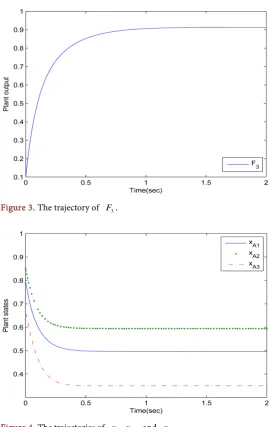
Figure 3. The trajectory of F3.

[image:16.595.239.511.70.265.2]

Figure 4. The trajectories of xA1,xA2 and xA3.

[image:17.595.239.514.68.256.2]

DOI: 10.4236/am.2017.812131 1848 Applied Mathematics

Figure 6. The trajectories of T T1, 2 and T3.

[image:17.595.237.518.72.719.2]

Figure 7. The trajectories of Q Q1, 2 and Q3.

DOI: 10.4236/am.2017.812131 1849 Applied Mathematics input reduce and tend to be stable gradually. From the results, we know the proposed output feedback distributed model predictive control architecture guarantees the ultimately boundedness of the system’s states, and then the reac-tor-separator process is stable.

7. Conclusion

For a class of nonlinear systems whose states are immeasurable, an output feed-back distributed model predictive control algorithm is proposed. The main idea is: For the considered system, when the outputs are sampled asynchronously, by introducing a state observer, the estimated states of the original system are ob-tained. It is proved that the error is bounded and the estimated states are ulti-mately bounded. The stability of closed-loop system is guaranteed and the per-formance of the closed-loop system is improved. The simulation results verify the effectiveness of the method proposed in this paper.

Acknowledgements

This research was supported by the Natural Science Foundation of China (61374004, 61773237, 61473170) and Key Research and Development Programs of Shandong Province 2017GSF18116.

References

[1] Wang, W.L., Rivera, D.E. and Kempf, K.G. (2003) Centralized Model Predictive Control Strategies for Inventory Management in Semiconductor Manufacturing Supply Chains. American Control Conference, Denver, 4-6 June 2003, 585-590. [2] Liu, J.F., Muñoz de la Peña, D. and Christofides, P.D. (2009) Distributed Model

Predictive Control of Nonlinear Process Systems. AiChE Journal, 55, 1171-1184.

https://doi.org/10.1002/aic.11801

[3] Su, B.L., Li, S.Y. and Zhu, Q.M. (2009) Predictive Control of the Initial Stable Re-gion for Constrained Switched Nonlinear Systems. Science in China, 39, 994-1003. [4] Zhu, J. (2002) Intelligent Predictive Control and Its Application. Zhejiang

Univer-sity Press, Hangzhou.

[5] Kong, X.B. and Liu, X.J. (2014) Nonlinear Model Predictive Control for DFIG-Based Wind Power Generation. IEEE Transactions on Automation Science & Engineering, 11, 1046-1055. https://doi.org/10.1109/TASE.2013.2284066

[6] Camponogara, E., Jia, D., Krogh, B.H. and Talukdar, S. (2002) Distributed Model Predictive Control. IEEE Control Systems, 22, 44-52.

https://doi.org/10.1109/37.980246

[7] Zhang, L.W. and Wang, J.C. (2012) Distributed Model Predictive Control with a Novel Partition Method. Proceedings of 31st Chinese Control Conference, Hefei, 25-27 July 2012, 4108-4113.

[8] Gao, Y.L., Xia, Y.Q. and Dai, L. (2015) Cooperative Distributed Model Predictive Control of Multiple Coupled Linear Systems. IET Control Theorem & Applications, 9, 2561-2567. https://doi.org/10.1049/iet-cta.2015.0096

De-DOI: 10.4236/am.2017.812131 1850 Applied Mathematics

layed Measurements. Automatica, 46, 52-61.

https://doi.org/10.1016/j.automatica.2009.10.033

[10] Tran, T. and Quang, N.K. (2013) Distributed Model Predictive Control with Re-ceding-Horizon Stability Constraints. International Conference on Control, 80, 85-90.

[11] Zhang, L.W., Wang, J.C., Ge, Y. and Wang, B.H. (2014) Robust Distributed Model Predictive Control for Uncertain Networked Control System. IET Control Theorem & Applications, 8, 1843-1851. https://doi.org/10.1049/iet-cta.2014.0311

[12] Álvarez, A., Ridao, M.A., Ramirez, D.R. and Sánchez, L. (2013) Distributed Model Predictive Control Techniques Applied to an Irrigation Cannal. European Control Conference (ECC), 415, 3276-3281.

[13] Jia, Y.B. and Liu, X.J. (2014) Distributed Model Predictive Control of Wind and So-lar Generation System. Proceedings of the 33rd Chinese Control Conference, Nanj-ing, 28-30 July 2014, 7795-7799.

[14] Farina, M. and Scattolini, R. (2011) An Output Feedback Distributed Predictive Control Algorithm. 50th IEEE Conference on Decision and Control and European Control Conference, Orlando, 12-15 December 2011, 8139-8144.

https://doi.org/10.1109/CDC.2011.6160366

[15] Giselsson, P. (2013) Output Feedback Distributed Model Predictive Control with Inherent Robustness Properties. American Control Conference, Washington DC, 17-19 June 2013, 1691-1696. https://doi.org/10.1109/ACC.2013.6580079

[16] Copp, D.A. and Hespanha, J.P. (2014) Nonlinear Output-Feedback Model Predic-tive Control with Moving Horizon Estimation. 53rd IEEE Conference on Decision and Control, Los Angeles, 15-17 December 2014, 3511-3517.

https://doi.org/10.1109/CDC.2014.7039934

[17] Homer, T. and Mhaskar, P. (2015) Output Feedback Model Predictive Control of Stochastic Nonlinear Systems. American Control Conference, Chicago, 1-3 July 2015, 793-798. https://doi.org/10.1109/ACC.2015.7170831

[18] Khalil, H.K. (2011) Nonlinear Systems. 3rd Edition, Publishing House of Electronics Industry, Beijing.