Munich Personal RePEc Archive
Robustness and Stability of Limit Cycles
in a Class of Planar Dynamical Systems
Datta, Soumya
Faculty of Economics, South Asian University
June 2014
Online at
https://mpra.ub.uni-muenchen.de/56970/
Robustness and Stability of Limit Cycles in a Class
of Planar Dynamical Systems
Soumya Datta
∗Faculty of Economics, South Asian University, New Delhi, INDIA. Email:[email protected]
October 20, 2013
Abstract
Using a macroeconomic example, the paper proposes an algorithm to sym-bolically construct the topological normal form of Andronov-Hopf bifurcation. It also offers a program, using the Computer Algebra System ‘Maxima’, to apply this algorithm. In case the limit cycle turns out to be unstable, the possibilities of the dynamics converging to another limit cycle is explored.
Keywords: Andronov-Hopf bifurcation, Limit cycles
JEL classification: C62; C69
∗Parts of this paper are drawn from the author’s Ph.D. thesis, titledMacrodynamics of Financing
1
Introduction
The Andronov-Hopf bifurcation theorem is widely used to establish existence of limit cycles in economic systems.1
However, in addition to the existence conditions, the Andronov-Hopf bifurcation must satisfy the non-degeneracy condition in order to prevent the degeneration of these limit cycles.2
Further, the Andronov-Hopf bifurcation might either be supercritical or subcritical. As pointed out by (Benhabib & Miyao 1981, Kind 1999), these two possibilities might have different economic interpretations. The supercritical case corresponds to stable limit cycles surrounding an unstable fixed point, and hence might be interpreted as stylized business or growth cycles. The subcritical case, on the other hand, correspond to repelling closed orbit surrounding a fixed point which is still stable, and might be interpreted to be corresponding to the concept of corridor stability as developed by (Leijonhufvud 1973). A meaningful economic analysis of these limit cycles, therefore, requires a test for both non-degeneracy and stability.
We should point out here that numerically testing an Andronov-Hopf bifurca-tion point for non-degeneracy and stability is quite widespread in the literature in natural sciences. In fact, software packages like XPPAUT or MATCONT already in-corporate some of the standard algorithms for these tests. A substantial literature in economics, however, relies on symbolic computation. This is one of the reasons why the literature in economics often stops short of testing Andronov-Hopf bifurcation for non-degeneracy and stability. This is one of the concerns we attempt to address in this paper. With this objective, we use a method outlined by (Kuznetsov 1997) and (Edneral 2007) to symbolically compute the topological normal form for an Andronov-Hopf bifurcation in plane and test for non-degeneracy and stability of its limit cycles. A related issue which we also address in this paper is to explore whether, under certain conditions, there is a possibility of alternate stable limit cycles emerg-ing when the test for stability of the limit cycle from Andronov-Hopf bifurcation fails.
We use a macroeconomic model developed in Datta (2012) to illustrate our method. We contend that the choice of our model is without any loss of general-ity. The method developed here can easily be applied in similar economic models represented by a large class of planar dynamical systems.
1
See, for instance, (Asada & Yoshida 2003), (Asada, Chen, Chiarella & Flaschel 2006), (Barnett & He 1998), (Barnett & He 2006), (Benhabib & Nishimura 1979), (Benhabib & Miyao 1981), (Chiarella & Flaschel 2000), (Chiarella, Flaschel & Franke 2005), (Franke 1992), (Velupillai 2006) and (Minagawa 2007).
2
2
The Model
In the following sections, we use the planar dynamical system given below, repre-senting the macroeconomic model developed in (Datta 2012):
˙
g(t) =
a1g(t)−a2{g(t)} 2
−a3d(t) +a4
hg(t) ˙
d(t) = [b1g(t)−b2d(t) +b3]d(t)
(1)
where g ∈ [0, gmax] is the rate of investment (or the ratio of investment to capital
stock), gmax is the maximum possible rate of investment3 d is the debt-capital ratio
and a1, a2, a3, a4, b1, b2, b3 ∈ ]0,∞[ are composite parameters consisting of various
combination of various behavioral parameters. his a control parameter. In the model in Datta (2012), h represented the speed of adjustment of actual to the desired rate of investment; more generally, this might be interpreted as a parameter representing the speed of adjustment of the variable g.4
We note that the dynamical system represented by (1) has six steady states, which we refer to as Ei ¯gi,d¯i
,i∈[0,1]. A full list of these steady states is provided in appendix A. We further note that at most two of these steady states, E5 ¯g5,d¯5
and E6 g¯6,d¯6
, are economically meaningful, i.e. lies within real positive orthant. We further note the following:
Lemma 1. For the dynamical system represented by (1), the real positive orthant is invariant.
Proof. Provided in appendix B.
It follows from lemma 1 that since only dynamics strictly within the real positive orthant is economically meaningful, we focus our attention on only such trajectories and ignore other trajectories in the rest of our discussion. In other words, we only consider E5 and E6 for discussion, and do not discuss the other steady states in the
rest of this study.
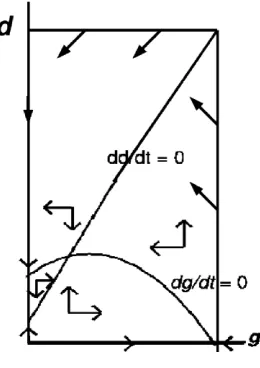
Next we turn our attention to the trajectories starting from an initial point inside the real positive orthant. Depending on the configuration of parameters, we can list four different possibilities exhibiting qualitatively different dynamics. These four cases are illustrated in figure 1. Details of parametric conditions giving rise to these four cases are discussed in appendix C.
3
In other words,gmax represents resource constraint commonplace in economic models. 4
Figure 1: Phase diagram of (1): Four cases
Further, performing the Routh-Hurwitz condition for local stability on the two economically meaningful steady states, E5 and E6, we note that (a) whenever
the non-trivial steady state solution, E5 exists and is distinct from E6 and lies in
the interior of real positive orthant, it is a saddle-point; and, (b) depending on the configuration of the parameters, the non-trivial steady state solution,E6, whenever it
exists and is distinct from E5 and lies within the interior of the real positive orthant,
is either a source or a sink.
3
Andronov-Hopf Bifurcation
Lemma 2. For an appropriate value of the speed of adjustment,h, of the actual rate of investment to its desired rate, the characteristic equation to (1) evaluated at the non-trivial steady state, E6, has purely imaginary roots.
E6, and recall that for case 1 of figure 1, ¯g6 >0, ¯d6 >0 anda1 −2a2¯g6 >0, so that
∂(Trace)
∂h = (a1−2a2g¯6) ¯g6 >0 (2)
i.e. the trace is smooth, differentiable and monotonically increasing in the speed of adjustment, h, of the actual to the desired rate of investment. We further note that the trace disappears at h = ˆh, when
(a1−2a2g¯6) ˆhg¯6−b2d¯6 = 0
⇒ ˆh= b2d¯6 (a1−2a2g¯6) ¯g6
>0 (3)
which, by substituting the values of ¯g6 and ¯d6 from (6), might be expanded as
ˆ
h= b1b2√4a2b2
2a4−4a2b2a3b3+b2
1a23−2a1b1b2a3+a2
1b22+2a2b2
2b3−b21b2a3+a1b1b2
2 (2b1a3
−a1b2)√4a2b2
2a4−4a2b2a3b3+b2
1a23−2a1b1b2a3+a2
1b22−4a2b2
2a4+4a2b2a3b3
−2b21a23+3a1b1b2a3
−a21b22
(4)
We define ˆh as the critical value of the parameter, h, and investigate the properties of a solution trajectory to (1) around ˆh. Next, we apply the Andronov-Hopf Bifurcation Theorem to note the following:
Corollary 2.1. For the dynamical system represented by (1), h= ˆhprovides a point of Andronov-Hopf bifurcation.
Proof. From lemma 2, the characteristic equation to (1) has purely imaginary roots at h = ˆh. Further, the transversality condition is satisfied from (2). Hence, h = ˆh
provides a point of Andronov-Hopf bifurcation.
Lemma 3. For the dynamical system represented by (1), we can identify specific combination of parameter values for which the Andronov-Hopf bifurcation at h= ˆh is non-degenerate and supercritical (or subcritical), leading to emergence of unique and stable (or unique and unstable) limit cycles.
Proof. Provided in appendix D.
4
Global Stability Properties
We recall that for any (g◦, d◦)∈intℜ2
++as the initial point, the solution to (1)
is represented by Θ (t) = (g(t), d(t) ; g◦, d◦). We attempt in this section to find out
We define a set Q⊆int ℜ2
++ consisting of the rectangular area as follows:
Q={(g, d) :g ∈[0,g¯3], d∈[0, dmax]} (5)
where dmax = (b1/b2) ¯g3+ (b3/b2) =
b1
p
4a2a4+a21+ 2a2b3+a1b1
/(2a2b2). It
would be evident that dmax is the point of intersection of ˙d/d = 0 with the vertical
[image:7.595.252.382.248.432.2]straight line g = ¯g3 (See figure 2).
Figure 2: Invariant set Q
We further define QB ⊆ Q comprising the boundary of Q, such that QB =
{(g, d) : g = 0, d∈[0, dmax]} ∪ {(g, d) :g = ¯g3, d∈[0, dmax]} ∪ {(g, d) : g ∈[0,g¯3], d= 0} ∪
{(g, d) : g ∈[0,g¯3], d=dmax}. Next, we note the following:
Lemma 4. For the trajectoryΘ (t) = (g(t), d(t) ; g◦, d◦), the set Q as defined in (5)
is invariant.
Proof. Provided in appendix E.
Theorem 1. For any (g◦, d◦)∈int ℜ2
++, the trajectory, Θ (t) either approaches the
non-trivial steady state, E6, or is a limit cycle surrounding it.
Proof. First, suppose (g◦, d◦)∈intQ. We recall that for case 1 of figure 1, E
6 is the
unique steady state in the interior of the positive orthant, and is either a source or a sink. Equations (3) and (4) provide us with a condition to distinguish between the two. In other words, h <ˆhwill imply thatE6 is a sink; on the other hand, ifh >ˆh,
then the steady state E6 is a source, so that by Poincar´e-Bendixson Theorem there
must be a limit cycle surrounding E6. Next, consider (g◦, d◦) ∈ int
ℜ2 ++\Q
. By construction, Θ (t) will eventually enter Q. Subsequently, it will either converge to
One should note that the result contained in theorem 1 is robust. It is valid for all set of configuration of parameters where h > ˆh, i.e. the speed of adjustment of the actual to desired rate of investment, h, exceeds certain threshold level ˆh. It also pertains to any solution with an economically feasible set of initial points.
5
Multiple Limit Cycles
In section 3, we noted the emergence of limit cycle from Andronov-Hopf bi-furcation. We further noted that this limit cycle could be either attracting or re-pelling, depending on the configuration of the parameters. In case of a subcritical Andronov-Hopf bifurcation leading to repelling or unstable limit cycle, if the limit cycle is located within an invariant set, then, from Poincar´e-Bendixson Theorem we have possibilities of another limit cycle which is attracting.5
Consider, for instance, the non-trivial steady state, E6, located within an
in-variant set, Q, in figure 2. We recall that the steady state E6 is either a source
or a sink, depending on whether the value of the parameter, h, is greater than or less than the critical value, ˆh. We further note from corollary 2.1 that E6
un-dergoes a Andronov-Hopf bifurcation leading to emergence of a small amplitude limit cycle when the bifurcation parameter, h passes through its critical value, ˆ
h. Let Γh be this limit cycle. Since Γh ∈ Q, it follows from the Jordan curve theorem6
that Q is separated into two sets – a compact set, A(Γh), comprising the area enclosed by Γh such that A(Γh) ⊆ Q, and, the half-open bounded set
Q\A(Γh) ≡ {(g, d) : (g, d)∈Q & (g, d)∈/ A(Γh)}. A(Γh) is bounded by Γh, the limit cycle resulting due to Poincar´e-Andronov-Hopf bifurcation. Suppose further that the configuration of parameters is such that the Andronov-Hopf bifurcation is subcritical, so that Γh is repelling. Now we note the following:
Lemma 5. Q\A(Γh) is non-empty.
Proof. We recall that Q is a compact invariant set, bounded by QB, and that all trajectories with an initial point on QB such that g, d 6= 0 gets pushed towards interior of Q. In other words, QB cannot be the ω-limit set of any trajectory. Since Γh is a limit cycle, A(Γh) must be a proper subset of Q, so that Q \ A(Γh) is non-empty.
5
See Hofbauer & So (1990), Hsu & Hwang (1999) and Yuquan, Zhujun & Chan (1999) for practical examples of emergence of multiple limit cycles by this method.
6The Jordan Curve Theorem.
Let C be a simple closed curve in S2
. Then C separates
S2
precisely into two components W1 and W2. Each of the sets W1 and W2 has C as its
Lemma 6. For Θ (t) = (g(t), d(t) ; g◦, d◦), Q\A(Γ
h) is invariant.
Proof. Consider a trajectory, Θ (t) starting from an initial point, (g◦, d◦)∈Q\A(Γ
h). We have already established, from lemma 4 that for all (g◦, d◦) ∈ Q the solution
trajectory, Θ (t) cannot cross QB. We further note that, since Γh is repelling, for all (g◦, d◦) ∈ Q\A(Γ
h), Θ (t) cannot cross Γh. Since Q\A(Γh) is constructed on a plane, the solution needs to cross either QB or Γh in order to leave Q\A(Γh). Hence, Q\A(Γh) is invariant.
Theorem 2. If the steady state E6 undergoes a subcritical Poincar´e-Andronov-Hopf
bifurcation at the critical value of the bifurcation parameter,ˆh, then as the bifurcation parameter hpasses throughˆh, in addition to the small amplitude unstable limit cycle,
Γh, there exists at least one large amplitude limit cycle which is attracting.
Proof. We note that, by construction, Q\A(Γh) contains no locally stable fixed point. Hence, from Poincar´e-Bendixson Theorem, for any (g◦, d◦) ∈ Q\A(Γ
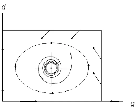
[image:9.595.194.454.487.696.2]h), ω -limit set of the solution trajectory, Θ (t) will be a closed orbit. Further, the limit cycle, Γh, emerging from Andronov-Hopf bifurcation as the bifurcation parameter passes through its critical value is not contained in Q\A(Γh), i.e. Γh ∈/Q\A(Γh). Hence, theω-limit set of Θ (t) must be a large amplitude limit cycle which is distinct from Γh. We further note that this large amplitude limit cycle is attracting. (See figure 3)
It is clear from theorem 2 that in case of a subcritical Andronov-Hopf bifurca-tion, the following two kinds of trajectories would emerge:
1. For any (g◦, d◦)∈intA(Γ
h) theω-limit set of the solution trajectories would be the steady state, E6. This behavior would be similar to Leijonhufvud’s (1973)
notion of corridor stability.
2. For any (g◦, d◦)∈Q\A(Γ
h), theω-limit set of the solution trajectories would be a large amplitude limit cycle.
In other words, a subcritical Andronov-Hopf bifurcation leads to possibilities of emergence of multiple limit cycles.
6
Conclusions
The above discussion leads us to the following conclusions:
1. For the dynamical system represented by (1), we define a critical value of the parameter h given by ˆh where we have a non-degenerate Andronov-Hopf bifurcation, leading to emergence of limit cycles.
2. The limit cycle emerging from Andronov-Hopf bifurcation is either stable or unstable; in case it is unstable, from theorem 2, we have another stable limit cycle enclosing the unstable limit cycle.
3. Forh >ˆh, from theorem 1, we have a stable limit cycle from an application of Poincar´e-Bendixson theorem.
In other words, given ˆh, we have established the existence of a unique stable limit cycle for allh≥ˆh. We should note that this result for existence of stable limit cycles in planar dynamical systems is more robust than much of the current literature.
Appendix A
Steady states
The steady states of the dynamical system represented by (1) are as follows:
E1 : ¯g1,d¯1
= (0,0) (6a)
E2 : ¯g2,d¯2
=
− √
4a2a4+a21−a1
2a2 ,0
(6b)
E3 : ¯g3,d¯3
=
√
4a2a4+a21+a1
2a2 ,0
(6c)
E4 : ¯g4,d¯4
=0,b3
b2
(6d)
E5 : ¯g5,d¯5
=
− √4
a2b22a4−4a2b2a3b3+b21a23−2a1b1b2a3+a21b22+b1a3−a1b2
2a2b2 ,
−b1√4a2b22a4−4a2b2a3b3+b21a23−2a1b1b2a3+a21b22−2a2b2b3+b21a3−a1b1b2
2a2b22
(6e)
E6 : ¯g6,d¯6
=
√
4a2b22a4−4a2b2a3b3+b21a23−2a1b1b2a3+a21b22−b1a3+a1b2
2a2b2 ,
b1√4a2b22a4−4a2b2a3b3+b21a23−2a1b1b2a3+a21b22+2a2b2b3−b21a3+a1b1b2
2a2b22
(6f)
It would be evident that E2 ∈ ℜ/ 2++ since ¯g2 < 0. Hence we do not discuss E2 any
further in the following sections. Further,E3 andE4 are non-negative and lie on the
g and d axis respectively. Regarding E5 and E6, we note the following:
1. Whenever E5 and E6 are real and distinct, ˙d/d = 0 must intersect ˙g/g = 0
from above at E5 and from below at E6. If E5 and E6 are not distinct, then
˙
d/d= 0 is a tangent to ˙g/g = 0 at the point representing the unique non-trivial steady state.
2. a3b3 < a4b2 is a sufficient (though not necessary) condition for the non-trivial
steady state E6 to be inside the real positive orthant, ℜ2++.
3. Forg(t)≥¯g3, we have ˙g(t)≤0 for all d(t)∈ ℜ+; in other words, if ¯g3 ≤gmax,
then the feasibility condition 0≤g(t)≤gmax is always satisfied.
Appendix B
Proof of Lemma 1
For any (g◦, d◦) ∈ int ℜ2
++ as the initial point, let the solution to (1) be
about the behavior of trajectories in case the initial point is on one of the axes:
(a) ˙g >0, d˙= 0 ∀ {(g◦, d◦) : g◦ ∈]0,g¯
3[, d◦ = 0} as the initial point.
(b) ˙g <0, d˙= 0 ∀ {(g◦, d◦) : g◦ ∈]¯g3,∞[, d◦ = 0} as the initial point.
(c) ˙g = 0, d >˙ 0∀
(g◦, d◦) : g◦ = 0, d◦ ∈0,d¯4 as the initial point.
(d) ˙g = 0, d <˙ 0∀
(g◦, d◦) : g◦ = 0, d◦ ∈d¯4,∞ as the initial point.
(7)
i.e. both the g-axis and the d-axis are trajectories. Since trajectories cannot cross each other, this would make the real positive orthant invariant, i.e. trajectories starting from an initial point in the real positive orthant will always remain within it.
Appendix C
Parametric conditions for four cases
of Figure 1
For g, d6= 0, from (1) we have
˙
g(t)⋚0 ⇔ d(t)R a1
a3
g(t)− a2
a3 {
g(t)}2+a4
a3
˙
d(t)⋚0 ⇔ d(t)R b1
b2
g(t) +b3
(8)
Depending on the configuration of parameters, we can list four different possibilities exhibiting qualitatively different dynamics:
1. Case 1: Here, a4b2 −a3b3 > 0, i.e. intercept of ˙g/g = 0 is greater than that
of ˙d/d = 0, and b1/b2 > (a1−2a2g¯6)/a3 > 0, i.e. ˙d/d = 0 intersects ˙g/g = 0
from below in the positively sloped section of the latter curve. E6 ∈intℜ2++ is
the only steady state in this case inside the real positive orthant.
2. Case 2: Here, a4b2 −a3b3 > 0, i.e. intercept of ˙g/g = 0 is greater than that
of ˙d/d = 0, but unlike case 1, (a1−2a2g¯6)/a3 < 0 < b1/b2, i.e. ˙d/d = 0
intersects ˙g/g = 0 from below in the negatively sloped section of the latter curve. E6 ∈intℜ2++ is the unique steady state inside the real positive orthant.
3. Case 3: Here, a4b2 −a3b3 < 0, i.e. intercept of ˙g/g = 0 is less than that
of ˙d/d = 0, and (a1−2a2g¯5)/a3 > b1/b2 > 0 > (a1−2a2g¯6)/a3, i.e. ˙d/d = 0
intersects ˙g/g = 0 from below atE5when the latter is sloping upward, and from
above atE6when the latter is sloping downward. In this case,E5, E6 ∈intℜ 2 ++,
i.e. ˙d/d= 0 intersects ˙g/g = 0 twice in the interior of the real positive orthant.
4. Case 4: Here, a4b2 −a3b3 < 0, i.e. intercept of ˙g/g = 0 is less than that of
˙
steady state in the interior of the real positive orthant. Since we are interested in only the real positive orthant, we do not discuss case 4 any further in the rest of our discussion.
Appendix D
Proof of Lemma 3
In order to establish that this Andronov-Hopf bifurcation point is non-degenerate, and to determine the stability of the limit cycles emerging from this bifurcation, we reduce our dynamical system represented by (1) to its topological normal form, us-ing a method outlined by (Edneral 2007), (Wiggins 1990) and (Kuznetsov 1997, Kuznetsov 2006). We implement this method by writing a program, using com-puter algebra system Maxima (see program 1 in appendix F). The actual algorithm consists of the steps given below:
1. We perform a linear transformation of coordinates from (g(t), d(t)) to the new plane, (x1(t), x2(t)) such that g(t) =x1(t) + ¯g6, and d(t) =x2(t) + ¯d6.
With this shift, the steady state, E6 : ¯g6,d¯6
is placed at the origin, and the dynamical system (1) can be represented as
˙
x1(t) = h
−a2{x1(t)} 3
+a6{x1(t)} 2
+a5x1(t)−a3x1(t)x2(t)−a7x2(t)
˙
x2(t) = b4x1(t) +b1x1(t)x2(t)−b5x2(t)−b3{x2(t)} 2
(9) where
a5 =
2b1a3s1−a1b2s1−4a2b22a4+ 4a2b2a3b3−2b21a 2
3 + 3a1b1b2a3−a21b 2 2
2a2b22
a6 =−
3s1−3b1a3 +a1b2
2b2
a7 =
a3 (s1−b1a3+a1b2)
2a2b2
b4 =
b1 (b1s1+ 2a2b2b3−b21a3+a1b1b2)
2a2b22
b5 =
b1s1+ 2a2b2b3 −b21a3+a1b1b2
2a2b2
s1 =
q
4a2b22a4−4a2b2a3b3+b21a 2
3−2a1b1b2a3+a21b 2 2
2. For the transformed dynamical system represented by (9), we take a Taylor se-ries expansion around the steady state represented by the origin. The resulting expression can be represented in matrix notation as
˙
where X = x1
x2
!
is a column vector of the two variables, and A(h) is the
jacobian matrix so that A(h)X represents the linear part of the Taylor series expansion, i.e.
A(h) = a5h −a7h
b4 −b5
!
(11)
and F (X, h) represents the non-linear terms of the Taylor series expansion, starting with at least quadratic terms, such that F (X, h) = O(||x| |2
) +
O(||x| |3
) +. . .
3. Next, we calculate the eigenvalues, ϑ(h) and ϑ(h) of the jacobian matrix,
A(h) from (11):
ϑ(h), ϑ(h) = 1 2
(a5h−b5)±
q
a2 5h
2+ (2a
5b5−4a7b4) +b25
so that real part of the eigenvalues is expressed as Reϑ(h) =a5h−b5. Further,
d(Re ϑ(h))
dh
h=0
=a5 >0
i.e. transversality condition is satisfied.
4. We now recalculate the critical value, ˆh, of the bifurcation parameter, h. This would correspond to the right hand side of (4), expressed in terms of the new parameters defined above. Thus, we have
ˆ
h= b5
a5
(12)
Substituting the value of ˆh from (12) into (11), we have the jacobian at the critical value of bifurcation parameter:
Aˆh=
b5 −
a7b5
a5
b4 −b5
(13)
Further, we have DeterminantAˆh= (b4b5a7)/a5−b25. We define ω such
that ω2
= DeterminantAˆh. We now express Aˆh from (13) in terms of ω.
Aˆh=
b5 −
a7b5
a5
a5(b25+ω 2
)
a7b5 −
b5
The eigenvalues of Aˆh evaluated at the critical value of the bifurcation
parameter can now be expressed as ϑˆh, ϑˆh=±ıω.
5. We now calculate the eigenvector of Aˆh with respect to ϑˆh and call it
q, where
q= ıa7b5ω+a7b
2 5
a5ω 2
+a5b 2 5
!
i.e. Aˆhq = ϑˆhq. It would be evident that eigenvector of Aˆh with
respect to ϑˆh would be q, where q is the complex conjugate of q, so that
Aˆhq=ϑˆhq.
6. We next calculate AT ˆh, the transpose ofAˆh:
AT hˆ=
b5
a5(b25 +ω 2
)
a7b5
−aa7b5
5 −
b5
(15)
We note that the eigenvalues of AT ˆh would be the same as those of Aˆh
and might be represented as ϑhˆ and ϑˆh.
7. We next calculate the eigenvector of AT ˆhwith respect toϑˆh and call it
p, i.e.
p=
1
a7b5
ıa5ω−a5b5
i.e. AT ˆhp=ϑˆhp. It would be clear that the eigenvector ofAT ˆhwith
respect to ϑˆhwould be p, i.e. AT ˆhp=ϑhˆp.
8. We note that the scalar product ofp and q is given by
hp, qi= 2ıa7b
2
5ω−2a7b5ω 2
b5 +ıω
by multiplying the column vectorp with the reciprocal of the conjugate of the scalar product of p and q, i.e.
ˆ
p≡p. 1
hp, qi
This leaves us with the following:
ˆ
p=
ıω−b5
2a7b5ω2+ 2ıa7b25ω
1
2a5ω2+ 2ıa5b5ω
(16)
We now note that hp, qˆ i= 1.
9. Next, we perform a complex linear transformation, z = hp, xˆ i so that x =
zq+zq. We should note that x = zq+zq ⇔ hp, xˆ i = zhp, qˆ i+zhp, qˆ i ⇔
hp, xˆ i = z [∵hp, qˆ i= 1, hp, qˆ i= 0]. The transformation from (x1, x2) to z
might be viewed as a combination of two transformations, y = T (h)x and
z =y1+ıy2. It would be clear that the components (y1, y2) are the coordinates
of (x1, x2) in the real eigenbasis ofA(h) composed by (2Req,−2Imq). In this
basis, the matrix A(h) has its canonical real (Jordan) form
J(h) =T (h)A(h)T−1
(h) = Reϑ(h) −ω(h)
ω(h) Re ϑ(h)
!
This complex linear transformation imposes a linear relationship between (x1, x2)
and the real and imaginary parts ofz. With this transformation, the dynamical system represented by (9) is now reduced to a single differential equation:
˙
z =ϑ(h)z+g(z, z, h) (17)
where g(z, z, h) =hp(h), F(zq(h) +zq(h), α)i.
To perform this transformation, we first represent the right hand side of (9) by F1(x1, x2) andF2(x1, x2) respectively. Next, we make the following
substi-tution:
x1 =zq1+wq1 = (a7b25+a7b5ıω)z+ (a7b52−a7b5ıω)w
x2 =zq2+wq2 = (a5b25+a5ω2) (z+w)
(18)
instance, Kuznetsov 1997, page 103, footnote 5). Substituting from (18), we have
F1(zq1 +wq1, zq2+wq2)
= b5
a5
−a3
ıa7b5ω+a7b 2 5
z+ a7b 2
5−ıa7b5ω
w a5ω 2
+a5b 2 5
(z+w)
−a7 a5ω 2
+a5b 2 5
(z+w)−a2
ıa7b5ω+a7b 2 5
z+ a7b 2
5−ıa7b5ω
w 3
+a6
ıa7b5ω+a7b 2 5
z+ a7b 2
5−ıa7b5ω
w 2+a5
ıa7b5ω+a7b 2 5
z
+ a7b 2
5−ıa7b5ω
w
(19) and
F2(zq1+wq1, zq2+wq2)
= −b2
a5ω 2
+a5b 2 5
(z+w) 2+b1
ıa7b5ω+a7b 2 5
z+ a7b 2
5−ıa7b5ω
w
a5ω 2
+a5b 2 5
(z+w) −b5 a5ω 2
+a5b 2 5
(z+w) +b4
ıa7b5ω+a7b 2 5
z
+ a7b 2
5−ıa7b5ω
w
(20) We define a matrix F such that
F = F1(zq1+wq1, zq2 +wq2)
F2(zq1+wq1, zq2 +wq2)
!
(21)
and a new complex-valued function G(z, w) such that
G(z, w) =hp, Fˆ i (22)
where G can be calculated by a scalar multiplication of ˆp from (16) with F
from (21).7
10. Next, we calculate the First Lyapunov Exponent,ℓ1
ˆ
h as follows:
ℓ1
ˆ
h= 1
2ω2 Re ı
∂2 G ∂z2
z=0,w=0
∂2 G ∂z∂w
z=0,w=0
+ω ∂
3 G ∂z∂z∂w
z=0,w=0
!
(23)
The computer algebra system, Maxima, calculates the value of first Lyapunov exponent of our system as:
ℓ1
ˆ
h=− 1 2a2
5ω3
b5 b 2 5+ω
2
3a2a5a 2 7b
2 5ω
2
+a3a5a6a7b 2 5ω
2
−a3
5a7b1b2ω 2
−a2 3a 2 5b 2 5ω 2
−a3a 3 5b2b5ω
2
+ 2a4 5b
2 2ω
2
−2a2 6a
2 7b
4
5+a5a6a 2 7b1b
3 5+a
2 5a 2 7b 2 1b 2 5
+3a3a5a6a7b 4 5−3a
3
5a7b1b2b 2 5 −a
2 3a
2 5b
4 5−a3a
3 5b2b
3 5+ 2a
4 5b 2 2b 2 5 (24) 7
11. Once we have calculated the value of the First Lyapunov Exponent from (24) and established that it is non-zero (i.e. non-degeneracy conditions are sat-isfied), we can reduce (17) to its topological normal form using a series of transformations, including an invertible parameter-dependent shift of complex coordinates, a linear time rescaling and a non-linear time reparametrization, and elimination of terms of degree greater than four from the Taylor series (cf. Kuznetsov 1997, page 94-100). In this case, (17) can be represented in the topological normal form as:
˙
y1
˙
y2
!
= α −1
1 α
!
y1
y2
!
+̟ y2 1 +y
2 2
y1
y2
!
(25)
where ̟ = signℓ1
ˆ
h=±1,α = Re ϑ(h)
ω(h) ∈ ℜ and y = (y1, y2) T
∈ ℜ2
.
The normal form represented by (25) is locally topologically equivalent to the original dynamical system represented by (1) near the steady state,E6. For̟ = +1,
the normal form has a steady state at the origin, which is asymptotically stable for
α ≤0 and unstable forα >0; in the latter case, a unique and stable limit cycle with radius√αwill emerge. This is the case of a supercritical Andronov-Hopf bifurcation. Similarly, for ̟ = −1, the normal form has a steady state at the origin, which is asymptotically stable for α <0 and unstable forα≥0; in the former case, a unique and unstable limit cycle will emerge. This is the case of asubcritical Andronov-Hopf bifurcation.
Appendix E
Proof of Lemma 4
Consider a trajectory Θ (t) starting from an initial point located on the bound-ary, QB of Q, i.e. (g◦, d◦) ∈ QB. We recall from (7) that the g-axis and the d-axis are both trajectories. In particular, since E1(0,0) is a steady state,
(g◦, d◦) =E
1(0,0)⇒Θ (t) =E1(0,0) ∀ t∈ ℜ (26)
Since E3(¯g3,0) and E4 0,d¯4
are also steady states, by same logic,
(g◦, d◦) =E
3(¯g3,0) ⇒ Θ (t) =E3(¯g3,0) ∀ t∈ ℜ (27)
(g◦, d◦) = E
4 0,d¯4
⇒ Θ (t) =E4 0,d¯4
∀t ∈ ℜ (28)
In other words, if the initial point is either on E1, E2 orE3 then the trajectory will
remain at the initial point. Further, from (7), if the initial point is on either g-axis or
On the other hand, for (g◦, d◦) ∈ {(g, d) : g = ¯g
3, d∈]0, dmax[}, we have ˙g < 0 and
˙
d > 0 ; whereas for (g◦, d◦) ∈ {(g, d) :g ∈]0,g¯
3[} we have ˙g < 0 and ˙d < 0; i.e. in
both cases the trajectories would be pushed towards interior of Q. To summarize, for any (g◦, d◦) ∈ Q
B, the trajectories either remain on QB or are pushed towards the interior of Q; in no case do the trajectories leave Q. [See figure 2] In addition, since Q is constructed on a plane, i.e. Q⊆ ℜ2
++, no trajectory with an initial point
in the interior of Q can leave Q without crossing QB. This completes the proof of invariance of Q.
Appendix F
Program Code
The following program code is written for Maxima version 5.21.1, using Lisp SBCL 1.0.29.11.debian, distributed under the GNU Public License.
http://maxima.sourceforge.net
Program 1: To find first lyapunov exponent of Andronov-Hopf bifurcation F1 : ( a [ 1 ]∗g − a [ 2 ]∗g ˆ2 − a [ 3 ]∗d + a [ 4 ] )∗h∗g ;
F2 : ( b [ 1 ]∗g − b [ 2 ]∗d + b [ 3 ] )∗d ;
assume ( a [ 1 ]>0 , a [ 2 ]>0 , a [ 3 ]>0 , a [ 4 ]>0 , b [ 1 ]>0 , b [ 2 ]>0 , b [ 3 ]>0 , h>0 , g>0 , d>0)$
assume ( a [ 1 ]∗b [ 2 ] > a [ 3 ]∗b [ 1 ] )$ assume ( a [ 4 ]∗b [ 2 ] > a [ 3 ]∗b [ 3 ] )$ s o l : a l g s y s ( [ F1=0 , F2=0] , [ g , d ] )$ u : r h s ( s o l [ 6 ] [ 1 ] )$
v : r h s ( s o l [ 6 ] [ 2 ] )$
F3 : f u l l r a t s i m p ( s u b s t ( x [ 1 ] + u , g , F1 ) )$ F4 : f u l l r a t s i m p ( s u b s t ( x [ 1 ] + u , g , F2 ) )$ F5 : f u l l r a t s i m p ( s u b s t ( x [ 2 ] + v , d , F3 ) )$ F6 : f u l l r a t s i m p ( s u b s t ( x [ 2 ] + v , d , F4 ) )$ F7 : expand ( F5 ) ;
F8 : expand ( F6 ) ;
s1 : s q r t ( 4∗a [ 2 ]∗b [ 2 ] ˆ 2∗a [4]−4∗a [ 2 ]∗b [ 2 ]∗a [ 3 ]∗b [ 3 ] + b [ 1 ] ˆ 2∗a [ 3 ] ˆ 2
−2∗a [ 1 ]∗b [ 1 ]∗b [ 2 ]∗a [ 3 ] + a [ 1 ] ˆ 2∗b [ 2 ] ˆ 2 )$ F9 : s u b s t ( s , s1 , F7 ) ;
F10 : s u b s t ( s , s1 , F8 ) ;
cx1 : ( f a c t o r ( c o e f f ( F9 , x [ 1 ] ) + a [ 3 ]∗h∗x [ 2 ] ) ) / h $ cx12 : ( f a c t o r ( c o e f f ( F9 , x [ 1 ] ˆ 2 ) ) ) / h $
cx2 : ( f a c t o r ( c o e f f ( F9 , x [ 2 ] ) + a [ 3 ]∗h∗x [ 1 ] ) ) /h $
− a [ 7 ]∗x [ 2 ] − a [ 3 ]∗x [ 1 ]∗x [ 2 ] )∗h ) ;
r a t s i m p ( F9 − s u b s t ( [ a [ 5 ] = cx1 , a [ 6 ] = cx12 , a [ 7 ] = −cx2 ] , F11 ) ) ; dx1 : f a c t o r ( c o e f f ( F10 , x [ 1 ] ) − b [ 1 ]∗x [ 2 ] ) $
dx2 : f a c t o r ( c o e f f ( F10 , x [ 2 ] ) − b [ 1 ]∗x [ 1 ] ) $
F12 : f u l l r a t s i m p ( b [ 4 ]∗x [ 1 ] − b [ 5 ]∗x [ 2 ] − b [ 2 ]∗x [ 2 ] ˆ 2 + b [ 1 ]∗x [ 1 ]∗x [ 2 ] ) ;
r a t s i m p ( F10 − s u b s t ( [ b [ 4 ] = dx1 , b[5]=−dx2 ] , F12 ) ) ; J : j a c o b i a n ( [ F11 , F12 ] , [ x [ 1 ] , x [ 2 ] ] )$
J1 : s u b s t ( [ x [ 1 ] = 0 , x [ 2 ] = 0 ] , J )$ t r : m a t t r a c e ( J1 )$
h1 : s o l v e ( [ t r =0] , [ h ] )$
J2 : s u b s t ( [ h=r h s ( h1 [ 1 ] ) ] , J1 )$ %D el t a : det er mi na nt ( J2 )$
r u l e 1 : %omegaˆ2 = %D el t a $ m1 : s o l v e ( r u l e 1 , b [ 4 ] ) $ m: r h s (m1 [ 1 ] ) $
J3 : r a t s i m p ( s u b s t ( [ b [ 4 ] =m] , J2 ) ) ; Q: e i g e n v e c t o r s ( J3 ) ;
q : f u l l r a t s i m p ( denom (Q [ 3 ] [ 2 ] )∗ t r a n s p o s e (Q [ 3 ] ) ) ; J4 : t r a n s p o s e ( J3 )$
P : e i g e n v e c t o r s ( J4 ) ; p1 : t r a n s p o s e (P [ 2 ] )$ i n n e r p r o d u c t ( p1 , q )$
i n n e r : c o n j u g a t e ( i n n e r p r o d u c t ( p1 , q ) )$ p : f u l l r a t s i m p ( p1∗( 1 / i n n e r ) ) ;
i n n e r p r o d u c t ( p , q ) ;
F13 : s u b s t ( [ h=r h s ( h1 [ 1 ] ) ] , F11 )$ F14 : s u b s t ( [ h=r h s ( h1 [ 1 ] ) ] , F12 )$
CLT1 : x [ 1 ] = ( z∗q [ 1 ] + w∗( c o n j u g a t e ( q [ 1 ] ) ) ) [ 1 ] ; CLT2 : x [ 2 ] = ( z∗q [ 2 ] + w∗( c o n j u g a t e ( q [ 2 ] ) ) ) [ 1 ] ; F15 : s u b s t ( [ CLT1 , CLT2 ] , F13 ) ;
F16 : s u b s t ( [ CLT1 , CLT2 ] , F14 ) ; FF : ma t r i x ( [ F15 ] , [ F16 ] ) ;
G: i n n e r p r o d u c t ( p , FF ) ;
g1 : f u l l r a t s i m p ( d i f f (G, z , 2 ) )$
g [ 2 0 ] : f u l l r a t s i m p ( s u b s t ( [ z =0 , w=0] , g1 ) ) ; g3 : f u l l r a t s i m p ( d i f f (G, z , 1 ) )$
g4 : f u l l r a t s i m p ( d i f f ( g3 , w, 1 ) )$
g6 : f u l l r a t s i m p ( d i f f ( g1 , w, 1 ) )$
g [ 2 1 ] : f u l l r a t s i m p ( s u b s t ( [ z =0 ,w=0] , g6 ) ) ; c [ 1 ] : %i∗g [ 2 0 ]∗g [ 1 1 ] + %omega ∗ g [ 2 1 ] ;
l [ 1 ] : f a c t o r ( ( 1 / ( 2∗ %omega ˆ 2 ) ) ∗ r e a l p a r t ( c [ 1 ] ) ) ;
References
Asada, T., Chen, P., Chiarella, C. & Flaschel, P. (2006), ‘Keynesian dynamics and the wage-price spiral: A baseline disequilibrium model’, Journal of Macroeco-nomics 28(1), 90–130.
Asada, T. & Yoshida, H. (2003), ‘Coefficient Criterion for Four-dimensional Hopf Bifurcations: A Complete Mathematical Characterization and Applications to Economic Dynamics’, Chaos, Solitons and Fractals 18, 525–536.
Barnett, W. A. & He, Y. (1998), Bifurcations in Continuous-Time Macroeconomic Systems, Macroeconomics 9805018, EconWPA.
*http://ideas.repec.org/p/wpa/wuwpma/9805018.html
Barnett, W. & He, Y. (2006), Existence of Bifurcation in Macroeconomic Dynam-ics: Grandmont was Right, Working papers series in theoretical and applied economics 200610, University of Kansas, Department of Economics.
*http://ideas.repec.org/p/kan/wpaper/200610.html
Benhabib, J. & Miyao, T. (1981), ‘Some New Results on the Dynamics of the Gen-eralized Tobin Model’, International Economic Review 22(3), 589–96.
Benhabib, J. & Nishimura, K. (1979), ‘The Hopf Bifurcation and the Existence and Stability of Closed Orbits in Multisector Models of Optimal Economic Growth’,
Journal of Economic Theory 21, 421–444.
Chiarella, C. & Flaschel, P. (2000), The Dynamics of Keynesian Monetary Growth: Macro Foundations, Cambridge University Press.
Chiarella, C., Flaschel, P. & Franke, R. (2005), Foundations for a Disequilibrium Theory of the Business Cycle: Qualitative Analysis and Quantitative Assess-ment, Cambridge University Press, Cambridge, U.K.
Datta, S. (2012), Cycles and crises in a model of debt-financed investment-led growth, MPRA Paper 50200, University Library of Munich, Germany.
Edneral, V. F. (2007), An Algorithm for Construction of Normal Forms, in V. G. Ganzha, E. W. Mayr & E. V. Vorozhtsov, eds, ‘CASC’, Vol. 4770 of Lecture Notes in Computer Science, Springer, pp. 134–142.
Franke, R. (1992), ‘Stable, Unstable and Persistent Cyclical Behavior in a Keynes-Wicksell Monetary Growth Model’, Oxford Economic Papers 44, 242–256.
Hofbauer, J. & So, J. W. H. (1990), ‘Multiple Limit Cycles for Predator-prey Mod-els’, Mathematical Biosciences99(1), 71–75.
Hsu, S.-B. & Hwang, T.-W. (1999), ‘Hopf Bifurcation for a Predator-prey System of Holling and Leslie Type’, Taiwanese Journal of Mathematics 3(1), 35–53.
Kind, C. (1999), ‘Remarks on the Economic Interpretation of Hopf Bifurcations’,
Economics Letters 62, 147–154.
Kuznetsov, Y. A. (1997),Elements of Applied Bifurcation Theory, Vol. 112 ofApplied Mathematical Sciences, second edn, Springer-Verlag, New York.
Kuznetsov, Y. A. (2006), ‘Andronov-Hopf bifurcation’, Scholarpedia1(10), 1858. *http://www.scholarpedia.org/article/Andronov-Hopf bifurcation
Leijonhufvud, A. (1973), ‘Effective Demand Failures’,Swedish Journal of Economics 75, 27–48.
Minagawa, J. (2007), A determinantal criterion of Hopf bifurcations and its applica-tion to economic dynamics, in T. Asada & T. Ishikawa, eds, ‘Time and Space in Economics’, Springer, pp. 160–172.
Munkres, J. R. (2000), Topology, second edn, Pearson Education, Inc.
Velupillai, K. (2006), ‘A Disequilibrium Macrodynamic Model of Fluctuations’, Jour-nal of Macroeconomics 28(4), 752–767.
Wiggins, S. (1990), Introduction to Applied Nonlinear Dynamical Systems and Chaos, Springer-Verlag, New York, Inc.