3D Image Reconstruction using Raspberry Pi

3D Image Reconstruction using Raspberry Pi

Shruti Rayaji

M.Tech student, VLSI Design & Embedded Systems

Department of Electronics & Communications K.L.E. Dr. MSSCET, Belagavi, Karnataka

Udaykumar L. Naik, PhD

Professor, Department of Electronics & Communications

K.L.E. Dr. MSSCET, Belagavi, Karnataka

ABSTRACT

This paper proposes 3 dimensional image reconstruction captured of different objects angled differently. Raspberry Pi camera is used to capture the images. The main objective of this paper lies in using the two dimensional images in the form of cross sectional slides also known as multi slice-to-volume registration that are placed one above the other in a mesh to re-project it back to a three dimensional model. Iterative reconstruction algorithm is applied as it is insensitive to noise and even in case of incomplete data or image it helps in reconstructing the image in the most favorable manner. Finally, the experiments are compared with the other methods or algorithms such as Speeded up robust feature (SURF) and Sum of squared differences (SSD) methods which are far more complex with nominal clarity.

Keywords

Raspberry Pi; features; camera; 2d images; cross sectional; slice-to-volume registration; Iterative reconstruction.

1.

INTRODUCTION

We ask that authors follow some simple guidelines. In There has always been a demand for 3-dimensional image processing since beginning. With the growth in technology not just in the field of medical imaging but also in the area such as satellite imaging, military imaging for surveillance, Robotic guidance etc. the need of the same has even grown to greater heights. Methods such as multi slice-to-volume registration are applied to obtain the required 3d model. Each of the slice is formulated with a sparse matrix that merges with the sparse matrix of the consecutive slice to blend all the 1’s with the 1’s while the 0’s with the 0’s. The following consideration is made such as 0 as black and 1 as white. This results into a grey image. It also holds good for any colored image that lies in the range of Red, Green, and Blue (RGB). The most important criteria that lies here is matching of the key features of every input consecutive slices to formulate a final 3dimensional model. Due to multi images, the stereo Reconstruction Pipeline method is followed. Each of the plane obtained is placed at a fixed distance from each other and also from that of the object of interest. Hence depth calibration becomes one of the important factor. There is also disparity shift between every plane. Therefore, feature localization and depth computation is performed using traditional approach of using Epipolar geometry that describes the fundamental matrix that relates one image from the other that are placed at fixed distance and an angle between them[1].

2.

PROPOSED METHOD

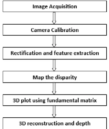
Fundamental matrix of the images is computed with the further aid of depth mapping. Image reconstruction is performed with the use of fundamental matrix of the image. Detailed discussion of the proposed technique is given below.

Figure 1- Block diagram of 3D image reconstruction

2.1

Image Acquisition

Figure 2- Skeletal representation of 10 cameras.

The following image gives the skeletal representation of the same.

Figure 3- Representation of multiview of 10 cameras.

2.2

Camera Calibration

The pin hole camera model given below is based on the principle of collinearity. [1]

Figure 4- Pin hole camera

As seen from the model a point in the space with coordinates is mapped with the point on the image plane. Hence the relationship between space coordinates and image plane as: x=PX with P being the projection matrix. Camera parameters are divided as intrinsic, extrinsic and distortion coefficients. With the help of the help of the available 2D and 3D image points we can estimate the camera parameters. The diagram below explains clearly that the camera parameters are represented in a 4-by-3 matrix called the camera matrix. Here the calibration algorithm is used to calculate the camera matrix using the extrinsic and intrinsic parameters. A virtual image plane is mapped by this matrix by using the 3D world scene. [1]

Figure 5- The intrinsic parameters include the optical center and focal length of the camera.

……….. (1)

where, w is the scale factor.

Left hand matrix indicates the image points

Right hand matrix indicates world points

P indicates the camera matrix nd is given by

………. (2)

Extrinsic Parameters basically consists of rotation and translation. While intrinsic parameters include focal length, optical center and skew coefficient. The intrinsic matrix is given by:

……… (3)

where, (fx, fy ) – are focal length in pixels and (Px , Py ) – are size of pixels world units.

2.3

Rectification and feature extraction

We follow the ORB (Oriented FAST and rotated BRIEF) algorithm which is a fast and a robust method of feature detector that was presented by Ethan Rublee et al. in 2011.

This fusion of FAST key point detector and BRIEF descriptor is used to improve the performance of the output 3d image by certain modifications. This method is considered as an efficient alternative to Scale-invariant feature transform (SIFT) or Speeded up robust feature (SURF) in 2011 also with respect to computation cost, matching performance and also patents it’s a very good alternative. It first starts with the use of Features from accelerated segment test(FAST) to find the key points and then applies Harris corner measure to find top N points among the images. It also produces multiscale-features by the use of pyramid.

2.4

Map the disparity

This helps in the mapping of the depth with the help of the stereo images. Here the concept of retinal disparity is used to observe the horizontal separation or the parallax that produces an illusion of one continuous image.

Figure 6- Depth mapping

From the above equivalent triangle the following equation for disparity is derived as follows:

Disparity=x-x’=Bf/Z……… (4)

where x and x’ represents the distance between points in image plane that corresponds to that of the scene points in the 3D and their corresponding camera center. B denotes the distance between two cameras and f the focal length of the camera that is known. Hence we can deduce that the depth of a point in a scene is inversely proportional to the difference in distance o corresponding image points and their respective camera centers. This in turn helps to evaluate the depth of all the pixels in an image [2].

2.5

3-Dimensional plot using fundamental

matrix

Fundamental matrix denoted by F is nothing but an algebraic representation of Epipolar geometry. Here, Epipolar geometry is the geometry of the intersection of the image planes with the pencil of planes having the line joining the camera centers known as the baseline. It helps in finding the corresponding points in the stereo matching [7].

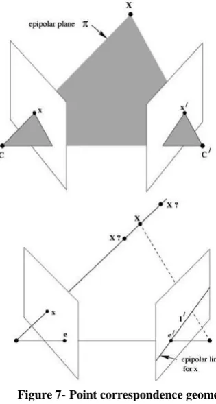
From the figure below, a point X in 3-space is imaged in two views, at x in the first and x’ in the next. The relationship between all of these is that they are coplanar. Let’s denote this plane as π. From the figure we can note that the rays projected from x and x’ intersect at X, and the rays are coplanar, lying in π. It is one of the most important property that is of most significance in searching for a correspondence.

Figure 7- Point correspondence geometry

 An Epipolar plane is a plane that contains the baseline as sown in the figure below. It includes one parameter family of Epipolar planes

 The Epipolar planes intersects the left image plane with that of the right planes in Epipolar lines, and defines the correspondence between the lines [8].

Figure 8- Representing the feature matching

For the geometric derivation of a fundamental matrix, the two images can be decomposed into two steps.

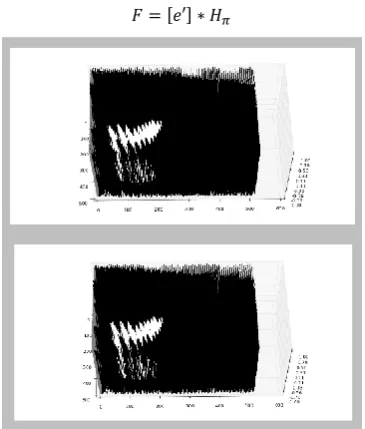
The first being that the point x is mapped to a corresponding point x’ on the other image that lies on the Epipolar line l’. Here x’ is known as the potential match for the point x. Hence fundamental matrix can be written as

Figure 10- Images obtained through fundamental matrix at 30 and 60 degree angle.

2.6 3-Dimension reconstruction and depth

From the above mentioned methodology a final 3D reconstruction mesh was applied on the figures captured. Following are the results of the 3D images obtained.

3.

EXPERIMENTAL RESULTS

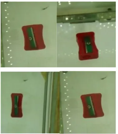
2D images of cashew and sharpener that are captured at different angles are shown in the figure 14 and figure 15 respectively. The following tabulations have been performed that gives the respective values of different parameters of these images. Such as aspect ratio which describes the proportional relationship between the width and height of an image. In the table1 we compute the aspect ratio of cashews and sharpener which is expressed as two numbers separated by a colon given as x : y. Similarly, it is evident from the table that the total area of the images is computed using their respective solidity, hull area, extent and perimeter values. These parameters prove to be of great importance in the reconstruction of the 3 dimensional image. Below are results and the outcome of the computation.

Figure 11- 3D reconstruction of images along with depth mapping

Figure 12- 3D image reconstruction of the images at 300.

Table 1

Images Area Perimeter

Aspect

Ratio Extent Hull Area Solidity

Equi

Diameter

Image Cashew -1 5.5 9.07 1.0 0.34 5.5 1.0 2.65

Image Cashew -2 13549 530.7 1.46 0.62 15509 0.8 131.3

Image Cashew -3 2.0 5.66 1.0 0.22 2.0 1.0 1.56

Image Cashew -4 13.0 16.46 2.0 0.41 14.5 0.89 4.07

Image Sharpner -1 6.5 15.41 0.25 0.41 6.5 1.0 2.88

Image Sharpner -2 3650.5 252.47 0.7 0.77 3910.5 0,93 68.2

Image Sharpner -3 7.0 16.0 0.25 0.44 7.0 1.0 2.99

Image Sharpner -4 2024.0 202.43 0.44 0.83 2242.5 0.9 50.76

Figure 14- 2D Images of Cashew captured at different angle

Figure 15- Images of Sharpener captured at different angle

4.

CONCLUSION AND FUTURE SCOPE

Auto image analysis is a complex task. Real time image capturing and converting them into 3D image is a very tedious task as it involves limiting of the tolerable error. In such a situation attempting to extract features is most intricate procedure. However, with the use of depth mapping and

formation of fundamental matrix as discussed above with the help of 2D images has produced good results. For the image reconstruction two different objects are considered. As seen from the table the area remains unique for different objects at different angle. As seen for cashew the area ranges between 2mm2 to 13549mm2 at varied angles. Similarly, for a sharpener it ranges between 6.5mm2 to 3650mm2. With the image sequencing of the fundamental matrix that is deduced it is possible achieve a 3D reconstruction up to an accuracy rate of 60% to 70%.

5.

ACKNOWLEDEGMENT

I take this opportunity to thank my college KLE’s. Dr.M.S.Sheshgiri college of Engineering & Technology. I would like to extend my profound thanks to Mr. Sasisekar; the founder of the company Nanopix pvt ltd, Hubli, without who’s support and concern this work would not have been completed.

6.

REFERENCES

[1] Zhang, Z. “A Flexible New Technique for Camera Calibration.” IEEE Transactions on Pattern Analysis and Machine Intelligence. Vol. 22, No. 11, 2000, pp. 1330–1334.

[2] Heikkila, J., and O. Silven. “A Four-step Camera Calibration Procedure with Implicit Image Correction.” IEEE International Conference on Computer Vision and Pattern Recognition.1997. [3] http://www.vision.caltech.edu/bouguetj/calib_docfor,

Camera Calibration

[4] Trucco, emanuele and verri, “Introductory Techniques for 3D Computer vision”.

[5] Viral H.Borisagar, Mukesh A.Zaveri, “A Novel Segment based Stereo Matching algorithm for Disparity map GenerationInternational conference on Computer and Software Modeling, Volume 14, 2011.

[6] Sahitya S, Lokesha H, Sudha L K “Real time application of Raspberry Pi in compression of images”, 2016 IEEE International Conference on Recent Trends in Electronics, Information & Communication Technology (RTEICT).

Computational Intelligence)2008 IEEE Congress on Evolutionary Computation (IEEE World Congress on Computational Intelligence)