Local Kernel Dimension Reduction in Approximate Bayesian Computation

ISSN Online: 2161-7198 ISSN Print: 2161-718X

Local Kernel Dimension Reduction in

Approximate Bayesian Computation

Jin Zhou, Kenji Fukumizu

Institute of Statistical Mathematics, Tachikawa, Japan

Abstract

Approximate Bayesian Computation (ABC) is a popular sampling method in applications involving intractable likelihood functions. Instead of evaluating the likelihood function, ABC approximates the posterior distribution by a set of accepted samples which are simulated from a generating model. Simulated samples are accepted if the distances between the samples and the observation are smaller than some threshold. The distance is calculated in terms of sum-mary statistics. This paper proposes Local Gradient Kernel Dimension Reduc-tion (LGKDR) to construct low dimensional summary statistics for ABC. The proposed method identifies a sufficient subspace of the original summary sta-tistics by implicitly considering all non-linear transforms therein, and a weighting kernel is used for the concentration of the projections. No strong assumptions are made on the marginal distributions, nor the regression mod-els, permitting usage in a wide range of applications. Experiments are done with simple rejection ABC and sequential Monte Carlo ABC methods. Results are reported as competitive in the former and substantially better in the latter cases in which Monte Carlo errors are compressed as much as possible.

Keywords

Approximate Bayesian Computation, Kernel Dimensional Reduction

1. Introduction

Monte Carlo methods are popular in sampling and inference problems. While the Markov Chain Monte Carlo (MCMC) methods find successes in applications where likelihood functions are known up to an unknown constant, MCMC cannot be used in scenarios where likelihoods are intractable. For these cases, if the problem can be characterized by a generating model, Approximate Bayesian Computation (ABC) can be used. ABC is a Monte Carlo method that approx-How to cite this paper: Zhou, J. and

Fu-kumizu, K. (2018) Local Kernel Dimension Reduction in Approximate Bayesian Com-putation. Open Journal of Statistics, 8, 479-496.

https://doi.org/10.4236/ojs.2018.83031

Received: February 26, 2018 Accepted: June 10, 2018 Published: June 13, 2018

Copyright © 2018 by authors and Scientific Research Publishing Inc. This work is licensed under the Creative Commons Attribution International License (CC BY 4.0).

http://creativecommons.org/licenses/by/4.0/

Open Access

imates the posterior distribution by jointly generating simulated data and para-meters and does the sampling based on the distance between the simulated data and the observation, without evaluating the likelihoods. ABC was first

intro-duced in population genetics [1] [2] and then been applied to a range of complex

applications including dynamical systems [3], ecology [4], Gibbs random fields

[5] and demography [6].

The accuracy of ABC posterior depends on sufficiency of summary statistics and Monte Carlo errors induced in the sampling. Given the generative model

(

|

)

p y θ _{of observation} y_obs with parameter

θ

_{, consider summary statistics}

(

)

obs s obs

s =G y and s G y= s

( )

, where G Ys: →S is the mapping from the

original sample space Y to low dimensional summary statistics S. The posterior

distribution, p

(

θ|yobs

)

, is approximated by p

(

θ|sobs

)

, which is constructed as p

(

θ|yobs

)

=

∫

pABC

(

θ, |s sobs

)

ds, with

(

, |

)

( ) (

|

)

(

)

,

ABC obs obs

p θ s s ∝p θ p s θ K s s− _{ (1)}

where K is a smoothing kernel with bandwidth . In the case of simple

rejec-tion ABC, K is often chosen as an indicator function I s s

(

− obs 

)

. If the

summary statistics s are sufficient, it can be shown that (1) converges to the

posterior p

(

θ|s_obs

)

as  goes to zero [7].

As shown above, the sampling is based on the distance between the summary statistics of the simulated sample s and the observation sobs. Approximation

er-rors are induced by the distance measure and are proportional to the distance threshold . It is desirable to set  as small as possible, but a small threshold

will increase the simulation time. This is a trade-off between the accuracy and the efficiency (simulation time). According to recent results on asymptotic

properties of ABC [8] [9], assuming that the summary statistics follow the

cen-tral limit theorem, the convergence rate of ABC when accepted sample size

N→ ∞ is depended on the behavior of µ =dN, where  is the threshold

above and the dN is defined as of same magnitude of eigen

( )

ΣN , the

eigen-values of the covariance matrix of the summary statistics as the function of N. In

practice, if a specific sampling method is chosen, the threshold  is constrained

by the computing resources and time, and thus can be accordingly determined. The design of summary statistics then remains the most versatile and difficult part in developing an efficient ABC algorithm. To avoid the “curse of dimensio-nality”, summary statistics should be low dimensional in addition of sufficiency. A vast body of literature of ABC has been published. Many are devoted to re-duce the sampling error by using more advanced sampling methods, from

sim-ple Rejection method [10], Markov Chain Monte Carlo (MCMC) [11] to more

sophisticated methods like sequential Monte Carlo [3] [12] and adaptive

sequen-tial Monte Carlo methods [13].

In this paper, we focus on the problem of summary statistics. In early works of ABC, summary statistics are chosen by domain experts in an ad-hoc manner. It is manageable if the dimensionality is small which the model is well understood by the experts. But choosing a set of appropriate summary statistics is much

more difficult in complex models. To address this problem, a set of redundant summary statistics are constructed as initial summary statistics; dimension re-duction methods are then applied yielding a set of low dimensional summary statistics while persevering the information.

Many dimension reduction methods have been proposed for ABC. Entropy based subset selection [14], partial least square [15], neural network [16] and

expected posterior mean [17] are a few of them. The entropy based subset

selec-tion method works well in instances where the set of low dimensional summary statistics is a subset of the initial summary statistics, but the computational com-plexity increases exponentially with the size of the initial summary statistics. The partial least square and neural network methods aim to capture the nonlinear relationships of the original summary statistics. In both cases, a specific form of

the regression function is assumed. A comprehensive review [18] discusses the

methods mentioned above and compares the performances. While the results are a mixed bag, it is reported that the expected posterior mean method

(Semi-automatic ABC) [17] produces relatively better results compared to the

methods mentioned above in various experiments. It is a popular choice also due to its simplicity.

Semi-automatic ABC [17] uses the estimated posterior mean as summary

sta-tistics. A pilot run of ABC is conducted to identify the regions of parameter space with non-negligible probability mass. The posterior mean is then esti-mated using the simulated data from that region and is used as the summary

sta-tistics in a formal run of ABC. A linear model of the form: ( )i

( )

i f i

θ =β y + is

used in the estimation, where f y

( )

are the possibly non-linear transforms of

the data. For each application, the features f y

( )

are carefully designed to

achieve a good estimation. In practice, a vector of powers of the data

(

_{y y y y, , , ,}2 3 4_

)

_{is often used as noted in [17].}

To provide a principled way of designing the regression function, capturing the higher order non-linearity and realizing an automatic construction of sum-mary statistics, we introduce the kernel based sufficient dimension reduction method as an extension of the linear projection based Semi-automatic ABC. This dimension reduction method is a localized version of gradient based kernel

di-mension reduction (GKDR) [19]. GKDR estimates the projection matrix onto

the sufficient subspace by extracting the eigenvectors of the kernel derivatives matrices in the reproducing kernel Hilbert spaces (RKHS). We give a brief re-view of this method in Section 2. In addition to the GKDR, in which the estima-tion averages over all data points to reduce variance, a localized GKDR is pro-posed by averaging over a small neighborhood around the observation in ABC. Each point is weighted using a distance metric measuring the difference between the simulated data and the observation. The idea is similar to role of the distance kernel function in (1). Another proposal is to use different summary statistics for different parameters. Note that sufficient subspace for different parameters can be different, depending on the particular problem. In these cases, applying

separated dimension reduction procedures yield better estimations of the para-meter.

The proposed method gives competitive results in comparison with

Semi-automatic ABC [17] when using simple rejection sampling. Substantial

improvements are reported in the sequential Monte Carlo cases, where threshold

 are pushed to as small as possible to isolate the performance of summary

sta-tistics from the Monte Carlo errors.

The paper is organized as follows. In Section 2, we review GKDR and intro-duce its localized modification followed by discussions of computation consid-erations. In Section 3, we show simulation results for various commonly con-ducted ABC experiments, and compare the proposed method with the Semi-automatic ABC.

2. Local Kernel Dimension Reduction

In this section, we review the Gradient based Kernel Dimension Reduction (GKDR) and propose the modified Local GKDR (LGKDR). Discussions are giv-en at the giv-end of this section.

2.1. Gradient based kernel Dimension Reduction

Given observation

(

s,θ

)

, where _s∈m _{are initial summary statistics and}

θ

∈ is the parameter to be estimated in a specific ABC application. Assuming

that there is a d-dimensional subspace _U⊂d_{, d m< such that}

T

| ,

s B s

θ⊥ (2)

where B=

(

β1, , βd

)

is the orthogonal projection matrix from m to d.

The columns of B spans U and T

d

B B=I . Condition (2) shows that given _{B s}T _,

θ

is independent of the initial summary statistics s. It is then sufficient to use d

dimensional constructed vector _{z B s=} T _{as the summary statistics. This}

sub-space U is called effective dimension reduction (EDR) space [20] in classical di-mension reduction literatures. While there are a tremendous amount of pub-lished works about estimating the EDR space, in this paper, we propose to use GKDR in which no strong assumption of marginal distribution or variable type is made. The following is a brief review of GKDR, and for further details, we re-fer to [19] [21] [22].

Let B=

(

β1, , βd

)

∈m d× be the projection matrix to be estimated, and

T

z B s= _{. We assume (2) is true and} p

₍

θ|s

₎

=p

₍

θ|z

₎

. The gradient of the re-gression function is denoted by ∇s as

(

|

)

(

|

)

(

|

)

s

E s E z E z

B

s s z

θ θ θ

∂ ∂ ∂

∇ = = =

∂ ∂ ∂ (3)

which shows that the gradients are contained in the EDR space. Given the fol-lowing estimator

T T

s s

M E= _∇ ∇ =_ BAB _,

where

(

_| T

) (

_| T

)

ij i j

A _{= }E E

θ β

s E

θ β

s __{, i j,} =_{1, ,}_d.

The projection directions

β

_{lie in the subspace spanned by the eigenvectors of}

M. It is then possible to estimate the projection directions using eigenvalue

de-composition. In GKDR, the matrix M is estimated by the kernel method

de-scribed below.

Let Ω be an non-empty set, a real valued kernel k:Ω × Ω →_{ is called}

positive definite if , 1

(

)

0

n

i j i j i j=c c k x x⋅ ≥

∑

for any xi∈Ω and ci∈. Given a

positive definite kernel k, there exists a unique reproducing kernel Hilbert space

(RKHS) H associated with it such that: (1) k x

( )

⋅, _{spans H; (2) H has the} re-producing property [23]: for all x∈Ω and f H∈ _, f k x,

( )

⋅, = f x

( )

_.

Given training sample

(

s1,θ1

)

, ,

(

sn,θn

)

,

let

(

_,

)

_exp

(

2 2

)

S i j i j S

k s s = − s s− σ and

(

_,

)

_exp

(

2 2

)

i j i j

kΘ θ θ = −θ θ− σΘ

be Gaussian kernels defined on _m _{and , associated with RKHS}

S

H and

HΘ, respectively. With assumptions of boundedness of the conditional

expecta-tion E

(

θ|S s=

)

and the average gradient functional with respect to z, the

functional can be estimated using cross-covariance operators defined in RKHS

and the consistency of their empirical estimators are guaranteed [22]. Using

these estimators, we construct a covariance matrix of average gradients as

( )

( ) (

T

)

1

(

)

1

( )

ˆ_{n i S i S n n S n n S i}

M s = ∇k s G +n I − G GΘ +n I − ∇k s (4)

where GS and GΘ are Gram matrices k s sS

(

i, j

)

and kΘ

(

θ θi, j

)

,

respective-ly. n m

S ×

∇k ∈ is the derivative of the kernel kS

( )

⋅,si with respect to si, and n

 is a regularization coefficient. This matrix can be viewed as the straight

for-ward extension of covariance matrix in principle component analysis (PCA); the data here are the features in RKHS representing the gradients instead of the gra-dients in their original real space.

The averaged estimator M =1n

∑

in=₁M sˆn

( )

i is calculated over the training sample

(

s1,θ1

)

, ,

(

sn,θn

)

. Finally, the projection matrix B is estimated by

tak-ing d eigenvectors corresponding to the d largest eigenvalues of M just like in

PCA, where d is the dimension of the estimated subspace.

2.2. Local Modifications

As discussed above, the estimator M is obtained by averaging over the

train-ing sample si. When applied to ABC, since only one observation sample is

available, we propose to generate a set of training data using the generating model and introduce a weighting mechanism to concentrate on the local region around the observation and avoid regions with low probability density.

Given simulated data X1, , XN and a weight kernel Kw:m→, we

propose the local GKDR estimator

( ) ( )

1

1 N _ˆ

w i i i

M K X M X

N =

=

∑

 ₍₅₎

where Mˆ is m m× _{matrix and} K X_w

_{( )}

_i is the corresponding weight.

( )

w

K x can be any weighting kernel. In the numerical experiments, a triweight

kernel is used, which is written as

( )

(

₂

)

3 2

1 2

1 , i obs

w i u

th obs

X X

K X u u

X X

<

−

= − =

− 1

where 1u<1 is the indicator function, and Xth is the threshold value which

de-termines the bandwidth. The normalization term of the triweight kernel is omit-ted since it does not change the eigenvectors we are estimating. The bandwidth

determined by Xth is chosen by empirical experiments and will be described in

0. The Triweight kernel is chosen for its concentration in the central area than other “bell shaped” kernels and works well in our experiments. Other distance metrics could be used instead of squared distance.

The idea of the proposed estimator is similar to the ABC estimator itself. Without the weighting and the concentration, the estimator will be averaged over all Xi, regardless of the distribution it is generated from. Since the basic

assumption of GKDR is that the response variable Y should come from the same

distribution, we cannot expect good result simply using all samples without proper weighting. The form of the estimator is the classic Nadaraya-Watson es-timator without normalization.

Description of LGKDR algorithm is given in Algorithm 1. Procedure

Gener-ate Sample is the algorithm to generGener-ate sample with parameter as input.

Proce-dure LGKDR is the algorithm to calculate matrix M X

( )

i as given in (4) and

(5).

Since the dimension reduction procedure is done before the sampling, it works as a pre-processing unit to the main ABC sampling procedure. It can be embodied in any ABC algorithm using different sampling algorithms. In this paper, the rejection sampling method is firstly employed for its simplicity and low computation complexity as a baseline. Further results on Sequential Monte Carlo ABC are also reported to illustrate the advantage of the purposed method.

Algorithm 1. LGKDR.

In these experiments, the distance thresholds are pushed to as small as possible to suppress the Monte Carlo errors and isolate the effects of summary statistics alone.

2.3. Separated Dimension Reduction

In some problems, not all summary statistics are necessary for every parameter.

For example, in the M/G/1 Queue model, the parameter θ3 that controls the

dis-tribution of the inter-arrival time are not related to the parameters θ1 and θ2,

which jointly determine the distribution of the service time. It can be expected that using different sets of summary statistics for θ3 with smaller dimensionality

would improve the sampling efficiency. To do that, the information that is unre-lated to the particular parameter is dropped in the dimensional reduction in ex-change of lower dimensionality. The experiments show that better results can be achieved using these settings.

More precisely, LGKDR incorporates information of θ in the calculation of

gradient matrix M . If θ is a vector, the relation of different elements of θ is

contained in the gram matrix Gθ as in (4). Separate estimations concentrate on

the information of the specific parameter rather than the whole vector. As shown in the experiments in Section 3.2, it can construct significantly more in-formative summary statistics in some problems by means of reducing estimation error.

For Semi-automatic ABC [17], the summary statistic for each parameter is the

estimated posterior mean, thus naturally separated. However, if these 1 dimen-sional vectors are used for each parameter separately, the results are not every

good. For best subset selection methods [15] [24], summary statistics are chosen

as the best subset of the original summary statistics using mutual information or sufficiency criterion. It can also be extended to a separated selection procedure. In LGKDR, we simply construct summary statistics by using only the particular parameter as the response variable.

2.4. Discussion on Hyper Parameters

In this section, we discuss the parameters for LGKDR. Parameters for the ABC sampling will be discussed in the experiments section.

First, the bandwidth of the weighting kernel affects the accuracy of LGKDR. By selecting a large bandwidth, the weights of directions spread out a larger re-gion around the observation points. A small bandwidth concentrates the weights on the directions estimated close to the observation sample. In our experiments, a bandwidth corresponding to an acceptance rate of approximately 10% gives a good result and is used throughout the experiments. The same parameter is set for the Semi-automatic ABC as well for the similar purpose. A more principled method for choosing bandwidth, like cross validation, could be applied to select the acceptance rate if the corresponding computation complexity is affordable.

The bandwidth of the Gaussian kernels σS, σΘ and the regularization

rameter n are crucial to all kernel based methods. The first two determine the

function spaces associated with the positive definite kernels and the latter affects

the convergence rate (see [25]). In this paper, cross validation is adopted to

se-lect the proper parameters. In the cross validation, for each set of candidate pa-rameters, the summary statistics are constructed using a simulated observation

,

obs sobs

θ _{, a training set}

(

θ_training,S_training

)

_{and a test set}

₍

θ_test,S_test

₎

. A small pilot run of rejection ABC is performed and the estimation of parameters are calcu-lated by kNN regression of θtest with the Stest. K is set to 5 in all cases. The

pa-rameters that yield the smallest least error between the θtest and θobs are

cho-sen. The final summary statistics are then constructed and passed to the formal run of ABC.

2.5. Computational Complexity

Computational complexity is an important concern of ABC methods. LGKDR requires matrix inversion, solving eigenvalue problems and the cross validation procedure. In this paper, training sample size are fixed to _{2 10×} 3 _{and 10}4 _for

LGKDR and Semi-automatic ABC, respectively. Under this setting, the total computational time of LGKDR are about 10 times over the linear regression. We believe that it is a necessary price to pay if the non-linearities between the sum-mary statistics are strong. Being unable to capture these information in dimen-sional reduction step will induce a poor sampling performance and a biased es-timation. Also, although the cross validation procedure takes the majority of computation time in LGKDR, it needs to be performed only once for each prob-lem. Once the parameters are chosen, the computation complexity of LGKDR is comparable to the linear-type algorithms. Overall, the computational complexity depends on both the dimensional reduction step and the sampling step. For complex models like population genetics, sampling is significantly more time consuming than the dimension reduction procedure.

3. Experiments

In this section, we investigate three problems to demonstrate the performance of LGKDR. Our method is compared to the classical ABC using initial summary

statistics and the Semi-automatic ABC [17] using estimated posterior means. In

the first problem, we discuss a population genetics model, which was investi-gated in many ABC literatures. We adopt the initial summary statistics used in

[26], and rejection ABC is used as the sampling algorithm. In the second

prob-lem, a M/G/1 stochastic queue model which was used in [16] and [17] are

dis-cussed. While the model is very simple, the likelihood function could not be tri-vially computed. In the last experiment we explore the Ricker model as discussed in [17] and [27]. The latter two problems are investigated by both Rejection ABC

and sequential Monte Carlo ABC method (SMC ABC) [13], the first problem is

omitted from SMC ABC because it involves repeated calling an outside program for simulation and is too time consuming for SMC ABC.

3.1. Implementation Details

The Rejection ABC is described in Algorithm 2 and the SMC ABC is shown in

Algorithm 3. The hyper-parameters used in LGKDR are set as discussed in

sec-tion 2.4. We use a modified code from [13] and R package “Easyabc” [28] in our

SMC implementation and would like to thank the corresponding authors. Gaus-sian kernels are used in all the LGKDR algorithms. The detailed specifications of Semi-automatic ABC will be described in each experiment.

For evaluation of the experiments conducted using rejection ABC, a set of

pa-rameters _θj _{where 1, ,}

obs

j∈ _ N _{and the corresponding observation sample}

j obs

Y are simulated from the prior and the conditional probability p Y

(

|θ

)

,

re-spectively, and are used as the observations. For each experiment, we fix the total

number of simulations N and the number of accepted sample Nacc. The sample

used for rejection are then generated and fixed for all three methods. Using this setting, although the randomness of the simulation program is contained in the sample; yet since the sample used for each method is same and fixed, we can ig-nore the randomness in the simulation program and compare the methods more fairly. Also, by using fixed set of sample, we can accurately set the acceptance rate for each method, which is the most influential parameter for the estimation accuracies. For evaluation, the Mean squared error (MSE) over the accepted pa-rameters ˆj

i

θ and observation _θj _{are defined as}

(

)

2

1

1 Nacc _ˆ

j j

j i

i acc

MSE

N = θ θ

 

= _ − _



∑



The Averaged Mean Square Error (AMSE) is then computed as the average

over MSEj of each observation pair

(

θj,Yobsj

)

as

1

1 Nobs _.

j j obs

AMSE MSE

N =

=

∑

It is used as the benchmark for Rejection ABC. Because of the difference of computation complexity, for fairness of comparison, the acceptance rates are set differently. For LGKDR, the acceptance rate is set to 1%; while for semi-automatic ABC and original ABC, the acceptance rates are set to 0.1%. The training sample and simulated sample are generated from the same prior and remain fixed.

Algorithm 2. Rejection-ABC.

Algorithm 3. Sequential-ABC.

For SMC ABC, to get to as small tolerance as possible, the simulation time is different for different method. AMSE is used as the benchmark for the accuracy of the queue model. In the case of Ricker model, due to the extremely long si-mulation time, only one observation is used and MSE is used instead in this case. Computation time is reported for both experiments.

3.2. Parameter Settings

Several parameters are necessary in running the simulations in ABC. For

Rejec-tion ABC, the total number of samples N and the accepted number of samples

acc

N are set before the simulation as mentioned above. For Semi-automatic

ABC and LGKDR, a training set needs to be simulated to calculate the projection matrix. For LGKDR, a further testing set is also generated for cross validation purposes. The value of these parameters is reported in the corresponding expe-riments. The simulation time for generating these sample set are negligible compared to the main ABC, especially in SMC ABC. For LGKDR, another

im-portant parameter is the target dimensionality D. There are no theoretically

sound methods available to determine the intrinsic dimensionality of the initial summary statistics. In practice, since the projection matrix is simply the

ex-tracted eigenvectors of the matrix M as in (5) ordered by the absolute value of

the corresponding eigenvalues, the dimensionality is just the number of the

genvectors been used. In our experiments, we run several rejection ABC proce-dures using different B on a small fixed test set, and then fix the dimensionality. Since the test set is fixed and the different projection matrices are directly ac-cessible, this procedure is very fast. A starting point can be set by preserving 70% of the largest eigenvalues in magnitude and it usually works well. There are a large collection of literatures on how to choose the number of principle

compo-nents in PCA, which is similar to our problem, for example, see [29] and

refer-ence therein.

3.3. Population Genetics

Analysis of population genetics is often based on the coalescent model [30]. A

constant population model is used in simple situations, where the population is assumed unchanged across generations. The parameter of interests in this case is

the scaled mutation rate θ, which controls the probability of mutation between

each generation. The detailed introduction of coalescent models can be found in

[31]. Various studies [11] [12] [32] have been conducted in population genetics

following different sampling algorithms. In this study, we adopt the setting of

kernel ABC [26] and compare the performance with ABC and Semi-automatic

ABC.

100 chromosomes are sampled from a constant population

(

N=10000

)

. The

summary statistics are defined using the spectrum of the numbers of segregating

sites, ssfs, which is a coarse-grained spectrum consisting of 7 bins based on the

Sturges formula

(

1 log+ 2Sseg

)

. The frequencies were binned as follows: 0% - 8%, 8% - 16%, 16% - 24%, 24% - 32%, 32% - 40%, 40% - 48% and 48% - 100%,

we use the uniform distribution θ~ 0,30

[

]

in this study rather than the

log-normal distribution in [26]. As ABC is often used for exploratory researches,

we believe that the performance based on an uninformative prior is important for evaluating summary statistics. The program package ms is used to generate

the sample, which is of common choice in literature of coalescent model [33].

We test 3 typical scaled mutation rates 5, 8 and 10 rather than random draws

from the prior. The results are averaged over 3 tests. A total number of 106

sam-ple is generated; 105 _{sample is generated as the training sample for LGKDR and}

Semi-automatic ABC. Different acceptance rates are set for different methods as

discussed above. We use ssfs as the summary statistics for both Semi-automatic

ABC and LGKDR. Local linear regression is used as the regression function for the former. In LGKDR, the dimension is set to 2.

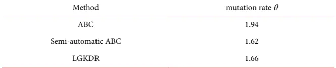
[image:11.595.207.540.652.720.2]

As shown in Table 1, the performance of both LGKDR and Semi-automatic

Table 1. Coalescent model.

Method mutation rate θ

ABC 1.94

Semi-automatic ABC 1.62

LGKDR 1.66

ABC improve over original ABC method. LGKDR and Semi-automatic ABC achieve very similar results suggesting that the linear construction of summary statistics is sufficient for this particular experiment.

3.4. M/G/1 Queue Model

The M/G/1 model is a stochastic queuing model that follows the first-come-first-serve principle. The arrival of customers follows a Poisson process with intensity

pa-rameter λ. The service time for each customer follows an arbitrary distribution

with fixed mean (G), and there is a single server (1). This model has an intracta-ble likelihood function because of its iterative nature. However a simulation

model with parameter

(

λ µ,

)

can be easily implemented to simulate the model.

It has been analyzed by ABC using various different dimension reduction

me-thods as in [16] and [17], with comparison to the indirect inference method. We

only compare our method with Semi-automatic ABC, since it produces substan-tially better results then the other methods mentioned above.

The generative model of the M/G/1 model is specified by

1

1 1

1 1

1 1 1 1

if if

n n

n i i i i

n _{n n n n}

n i i i i i i ii

U W Y

Y

U W Y W Y

−

= =

− −

= = = =

 _≤

 = 

+ − >



∑

∑

∑

∑

∑

∑

where Yn is the inter-departure time, Un is the service time for the nth

cus-tomer, and Wi is the inter-arrival time. The service time is uniformly

distri-buted in interval

[

θ θ1, 2

]

. The inter-arrival time follows an exponential

distribu-tion with rate θ3. These configurations stay the same as [16] and [17]. We set

uninformative uniform priors for θ θ θ1, 2− 1 and θ3 as

[

1,10

] [

2× 1,1 3

]

.

For the rejection ABC, we simulate a set of 30 pairs of

(

θ θ θ1, ,2 3

)

but avoid

boundary values. They are used as the true parameters to be estimated. The total

number of 106 _{sample are generated. The posterior mean is estimated using the}

empirical mean of the accepted sample. The simulated sample is fixed across different methods for comparison.

We use the quantiles of the sorted inter-departure time Yn as the exploration

variable of the regression model f y

( )

as in [17]. The powers of the variables are not included as no significant improvements are reported. A pilot ABC pro-cedure is conducted using a fixed training sample set of size 104_{. Local linear}

re-gression is used rather than a simple linear rere-gression for better results. For LGKDR, we use the same quantiles as initial summary statistics for dimension reduction as in Semi-automatic ABC. The number of accepted training sample is

3

2 10× _{in for the LGKDR. The dimension is manually set to 4, as small as the}

performance is not degraded.

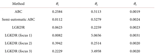
The experimental results of Rejection ABC are shown in Table 2. “LGKDR”

refers to the LGKDR that does not use separated estimation. “focus 1” denotes

the separated dimension reduction for parameter θ1, and the following rows are

of similar form. Compared to ABC, “Semi-automatic ABC” gives substantial

[image:13.595.212.540.90.208.2]

Table 2. M/G/1 queue model, rejection ABC.

Method θ1 θ2 θ3

ABC 0.2584 0.5113 0.0019

Semi-automatic ABC 0.0112 0.5279 0.0024

LGKDR 0.0623 0.2259 0.0023

LGKDR (focus 1) 0.0082 5.0656 0.0031

LGKDR (focus 2) 0.3942 0.2514 0.0020

LGKDR (focus 3) 0.2229 3.4958 0.0020

improvement on the estimation of θ1; the other parameters show similar or

slightly worse results. LGKDR method improves over ABC on θ1 and θ2, but the

estimation of θ1 is not as good as in Semi-automatic ABC. However, after

apply-ing separated estimation, θ1 presents a substantial improvement compared to

Semi-automatic ABC. Separated estimations for θ2 and θ3 give no improvements.

It suggests that the sufficient dimension reduction subspace for θ1 is different

from the others and a separated estimation of θ1 is necessary.

For SMC ABC, a set of 10 pairs of parameters are generated, and the results on SMC and LGKDR are reported. All other settings are same as the rejection ABC. We omit the results of using Semi-automatic ABC since the sequential chain did not converge properly using these summary statistics and the induced errors were too large to be meaningful. In SMC ABC, two experiments are

re-ported: SMC ABC1 and SMC ABC2. The number of particles are set to _{2 10×} 4

and 105_{, respectively. In LGKDR, the number of particles are set to 2 10×} 4 _and

the training sample size for the calculation of projection matrix is _{2 10×} 3_,

ac-cepted from a training set of size _{4 10×} 4_{. The dimensionality is set to 5. Cross}

validation is conducted using a test set of size _{2 10×} 4_.

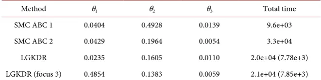
Results of SMC ABC are shown in Table 3. AMSEs are reported. The

simula-tion time is shown as well. The computasimula-tional time of constructing LGKDR summary statistics is included in the total simulation time and is listed in the

bracket. The results show that LGKDR gives better results of parameter θ1 and

θ2, using less time compared to SMC ABC with set E2. The estimation of θ3 is

worse but the difference is small (0.005). Focusing on θ3 produces an estimation

as good as in SMC ABC.

3.5. Ricker Model

Chaotic ecological dynamical systems are difficult for inference due to its dy-namic nature and the noises presented in both the observations and the process. Wood [27] addresses this problem using a synthetic likelihood inference

me-thod. Fearnhead [17] tackles the same problem with a similar setting using the

Semi-automatic ABC and reports a substantial improvement over other me-thods. In this experiment, we adopt the same setting and apply LGKDR with various configurations.

[image:14.595.208.539.89.172.2]

Table 3. M/G/1 queue model, SMC ABC.

Method θ1 θ2 θ3 Total time

SMC ABC 1 0.0404 0.4928 0.0139 9.6e+03

SMC ABC 2 0.0429 0.1964 0.0054 3.3e+04

LGKDR 0.0235 0.1605 0.0110 2.0e+04 (7.78e+3)

LGKDR (focus 3) 0.4854 0.1383 0.0059 2.1e+04 (7.85e+3)

A prototypic ecological model with Richer map is used as the generating

model in this experiment. A time course of a population Nt is described by

1 e N et t

t t

N rN − +

+ = (6)

where et is the independent noise term with variance σe2, and r is the growth

rate parameter controlling the model dynamics. A Poisson observation y is made

with mean φNt. The parameters to infer are θ=

(

log

( )

r , ,σ φe2

)

. The initial state is N0=1 and observations are y y51, 52, , y100.

The original summary statistics used by Wood [27] are the observation mean

y, auto-covariances up to lag 5, coefficients of a cubic regression of the ordered

difference y yt− t−1 on the observation sample, estimated coefficients for the

model 0.3 0.3 0,6

1 1 2

t t t t

y+ =β y +β y + and the number of zero observations

(

)

100

51 t 0

t= y =

∑

1 . This set is denoted as E0 as in [17]. Additional two sets of

sum-mary statistics are defined for Semi-automatic ABC. The smaller E1 contains E0 and

(

)

100 51 t

t= y = j

∑

1 for 1≤ ≤j 4_{, logarithm of sample variance,}

(

100

)

51

log j

t t= y

∑

for 2≤ ≤j 6 _{and auto-correlation to lag 5. Set E2 further includes}

time-ordered observation yt, magnitude-ordered observation

( )t

y , 2

t

y , y( )2t ,

{

log 1

(

+yt

)

}

,

{

log 1

(

+y( )t

)

}

,

time difference ∆yt and magnitude difference ∆y( )t . Additional statistics are

added to explicitly explore the non-linear relationships of the original summary statistics and are carefully designed.

In Rejection ABC, we use set E0 for ABC without dimension reduction since the dimension of the larger sets induces severely decreased performance. Sets E1

and E2 are used for Semi-automatic ABC as in [17]. In LGKDR, we tested sets

E0 and E1 in different experiments. The result on E2 is omitted as the result is similar with using the smaller set of statistics, indicating that manually designed non-linear features are unnecessary for LGKDR. The sufficient dimension is set to 5; a smaller value induces substantial worse results. We simulated a set of 30

parameters, a fixed simulated sample of size 107 _{for all the methods and a}

train-ing sample of size 106_{, a test sample of size 10}5 _{for LGKDR and Semi-automatic}

ABC. The values of log

( )

r and ϕ are fixed as in [17], and log

( )

σe are drawn from an uninformative uniform distribution on _log 0.1 ,0

( )

_.

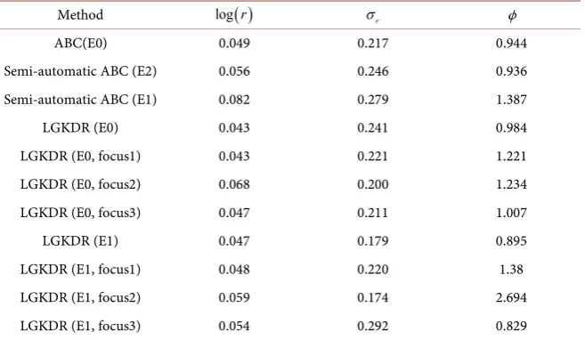
The results are shown in Table 4. The performance of Semi-automatic ABC

[image:15.595.212.541.89.280.2]

Table 4. Ricker model, rejection ABC.

Method log

( )

r σe ϕ

ABC(E0) 0.049 0.217 0.944

Semi-automatic ABC (E2) 0.056 0.246 0.936

Semi-automatic ABC (E1) 0.082 0.279 1.387

LGKDR (E0) 0.043 0.241 0.984

LGKDR (E0, focus1) 0.043 0.221 1.221

LGKDR (E0, focus2) 0.068 0.200 1.234

LGKDR (E0, focus3) 0.047 0.211 1.007

LGKDR (E1) 0.047 0.179 0.895

LGKDR (E1, focus1) 0.048 0.220 1.38

LGKDR (E1, focus2) 0.059 0.174 2.694

LGKDR (E1, focus3) 0.054 0.292 0.829

using the bigger set E2 is similar to ABC but is substantially worsen with set E1, suggesting that the non-linear information are essential for an accurate estima-tion in this model. These features are needed to be explicitly designed and in-corporated into the regression function for Semi-automatic ABC. LGKDR using summary statistics set E0 gives similar results compared with ABC. Using larger set E1, the accuracy of log

( )

r is slightly worse than using set E0, but the

accu-racy of σe and ϕ present substantial improvements. The additional gains of

separate constructions of summary statistics in this model are mixed for different

parameter, log

( )

r and ϕ show very small improvements but σe gets

im-provements in both cases. Overall, we recommend using separate constructions for the potential improvements if the additional computational costs are afford-able.

In SMC ABC, we use set E0 for the SMC, E1 for LGKDR and both E1 and E2

for Semi-automatic ABC. Number of particles is set to _{5 10×} 3 _{for all}

experi-ments. Other parameters are the same as in Rejection ABC. Only one set of pa-rameter is used and the time of simulation is set to achieve a tolerance which is as small as possible. Simulation time is reported with computational time of LGKDR included. We show several results with different settings of dimensio-nality in LGKDR to illustrate the influence of that hyper-parameter. As can be observed in the results, if the dimensionality is set too high, the efficiency of the SMC chain is decreased; if it is set too low, more bias are induced in the esti-mated posterior mean suggesting loss of information in the constructed sum-mary statistics. In this experiment, dimensionality 6 is chosen by counting the number of largest 70% eigenvalues in magnitude as discussed before.

The results are shown in Table 5. It shows that the LGKDR can achieve the

similar results as Semi-automatic ABC using only 1/10 of the simulation time.

4. Conclusions

We proposed the LGKDR algorithm for automatically constructing summary

[image:16.595.210.541.90.208.2]

Table 5. Ricker model, SMC ABC.

Method log

( )

r σe ϕ Total time

ABC(E0) 0.001 0.003 0.430 4.0e+5

Semi-automatic ABC(E2) 0.002 0.020 0.013 4.3e+5

Semi-automatic ABC(E1) 0.031 0.079 0.019 1.7e+5

LGKDR(Dimensional 3) 0.024 0.131 0.779 8.6e+4

LGKDR(Dimensional 6) 0.006 0.018 0.012 4.5e+4

LGKDR(Dimensional 9) 0.001 0.040 0.250 2.8e+5

statistics in ABC. The proposed method assumes no explicit functional forms of the regression functions and the marginal distributions, and implicitly incorpo-rates higher order moments up to infinity. As long as the initial summary statis-tics are sufficient, our method can guarantee to find a sufficient subspace with low dimensionality. While the involved computation is more expensive than the simple linear regression used in Semi-automatic ABC, the dimension reduction is conducted as the pre-processing step and the cost may not be dominant in comparison with a computationally demanding sampling procedure during ABC. Another advantage of LGKDR is the avoidance of manually designed fea-tures; only initial summary statistics are required. With the parameter selected by the cross validation, construction of low dimensional summary statistics can be performed as in a black box. For complex models in which the initial sum-mary statistics are hard to identify, LGKDR can be applied directly to the raw data and identify the sufficient subspace. We also confirm that construction of different summary statistics for different parameters improves the accuracy sig-nificantly.

Acknowledgements

Sincere thanks to the members of OJS for their professional performance, and special thanks to managing editor Alline Xiao for a rare attitude of high quality.

References

[1] Pritchard, J.K., Seielstad, M.T., Perez-Lezaun, A. and Feldman, M.W. (1999) Popu-lation Growth of Human Y Chromosomes: A Study of Y Chromosome Microsatel-lites. Molecular Biology and Evolution, 16, 1791-1798.

https://doi.org/10.1093/oxfordjournals.molbev.a026091

[2] Beaumont, M.A., Zhang, W. and Balding, D.J. (2002) Approximate Bayesian Com-putation in Population Genetics. Genetics, 162, 2025-2035.

[3] Toni, T., Welch, D., Strelkowa, N., Ipsen, A. and Stumpf, M.P. (2009) Approximate Bayesian Computation Scheme for Parameter Inference and Model Selection in Dynamical Systems. Journal of the Royal Society Interface, 6, 187-202.

https://doi.org/10.1098/rsif.2008.0172

[4] Csillry, K., Blum, M.G.B., Gaggiotti, O.E. and Franois, O. (2010) Approximate Bayesian Computation (ABC) in Practice. Trends in Ecology and Evolution, 25,

410-418. https://doi.org/10.1016/j.tree.2010.04.001

[5] Grelaud, A., Robert, C.P., Marin, J.M., Rodolphe, F. and Taly, J.F. (2009) ABC Like-lihood-Free Methods for Model Choice in Gibbs Random Fields. Bayesian Analysis, 4, 317-335. https://doi.org/10.1214/09-BA412

[6] Bertorelle, G., Benazzo, A. and Mona, S. (2010) ABC as a Flexible Framework to Es-timate Demography over Space and Time: Some Cons, Many Pros. Molecular Ecol-ogy, 19, 2609-2625. https://doi.org/10.1111/j.1365-294X.2010.04690.x

[7] Blum, M.G.B. (2010) Approximate Bayesian Computation: A Nonparametric Pers-pective. Journal of the American Statistical Association, 105, 1178-1187.

https://doi.org/10.1198/jasa.2010.tm09448

[8] Frazier, D.T., Martin, G.M., Robert, C.P. and Rousseau, J. (2016) Asymptotic Prop-erties of Approximate Bayesian Computation. ArXiv e-prints.

[9] Li, W. and Fearnhead, P. (2015) On the Asymptotic Efficiency of ABC Estimators. ArXiv e-prints.

[10] Moore, W.S. (1995) Inferring Phylogenies from Mtdna Variation-Mitochondrial-Gene Trees Versus Nuclear-Gene Trees. Evolution, 49, 718-726.

https://doi.org/10.2307/2410325

[11] Marjoram, P., Molitor, J., Plagnol, V. and Tavare, S. (2003) Markov Chain Monte Carlo without Likelihoods. Proceedings of the National Academy of Sciences of the United States of America, 100, 15324-15328.

[12] Sisson, S.A., Fan, Y. and Tanaka, M.M. (2007) Sequential Monte Carlo without Li-kelihoods. Proceedings of the National Academy of Sciences of the United States of America, 104, 1760-1765.https://doi.org/10.1073/pnas.0607208104

[13] Del Moral, P., Doucet, A. and Jasra, A. (2012) An Adaptive Sequential Monte Carlo Method for Approximate Bayesian Computation. Statistics and Computing, 22, 1009-1020.https://doi.org/10.1007/s11222-011-9271-y

[14] Joyce, P. and Marjoram, P. (2008) Approximately Sufficient Statistics and Bayesian Computation. Statistical Applications in Genetics and Molecular Biology, 7, Article 26.

[15] Wegmann, D., Leuenberger, C. and Excoffier, L. (2009) Efficient Approximate Bayesian Computation Coupled with Markov Chain Monte Carlo without Likelih-ood. Genetics, 182, 1207-1218.https://doi.org/10.1534/genetics.109.102509

[16] Blum, M.G.B. and Franccois, O. (2010) Non-Linear Regression Models for Ap-proximate Bayesian Computation. Statistics and Computing, 20, 63-73.

https://doi.org/10.1007/s11222-009-9116-0

[17] Fearnhead, P. and Prangle, D. (2012) Constructing Summary Statistics for Ap-proximate Bayesian Computation: Semi-Automatic ApAp-proximate Bayesian Com-putation. Journal of the Royal Statistical Society Series B: Statistical Methodology, 74, 419-474.https://doi.org/10.1111/j.1467-9868.2011.01010.x

[18] Blum, M.G.B., Nunes, M.A., Prangle, D. and Sisson, S.A. (2013) A Comparative Re-view of Dimension Reduction Methods in Approximate Bayesian Computation.

Statistical Science, 28, 189-208.https://doi.org/10.1214/12-STS406

[19] Fukumizu, K., Bach, F.R. and Jordan, M.I. (2004) Dimensionality Reduction for Supervised Learning with Reproducing Kernel Hilbert Spaces. Journal of Machine Learning Research, 5, 73-99.

[20] Li, K.C. (1991) Sliced Inverse Regression for Dimension Reduction. Journal of the American Statistical Association, 86, 316-327.

https://doi.org/10.1080/01621459.1991.10475035

[21] Fukumizu, K., Bach, F.R. and Jordan, M.I. (2009) Kernel Dimension Reduction in Regression. The Annals of Statistics, 37, 1871-1905.

https://doi.org/10.1214/08-AOS637

[22] Fukumizu, K. and Leng, C. (2014) Gradient-Based Kernel Dimension Reduction for Regression. Journal of the American Statistical Association, 109, 359-370.

https://doi.org/10.1080/01621459.2013.838167

[23] Aronszajn, N. (1950) Theory of Reproducing Kernels. Transactions of the American Mathematical Society, 68, 337-337.

https://doi.org/10.1090/S0002-9947-1950-0051437-7

[24] Nunes, M. and Balding, D.J. (2010) On Optimal Selection of Summary Statistics for Approximate Bayesian Computation. Statistical Applications in Genetics and Mo-lecular Biology, 9, Article 34.

[25] Smola, A.J., Schölkopf, B. and Müller, K.R. (1998) The Connection between Regula-rization Operators and Support Vector Kernels. Neural Networks, 11, 637-649. https://doi.org/10.1016/S0893-6080(98)00032-X

[26] Nakagome, S., Fukumizu, K. and Mano, S. (2013) Kernel Approximate Bayesian Computation in Population Genetic Inferences. Statistical Applications in Genetics and Molecular Biology, 12, 667-678.https://doi.org/10.1515/sagmb-2012-0050

[27] Wood, S.N. (2010) Statistical Inference for Noisy Nonlinear Ecological Dynamic Systems. Nature, 466, 1102-1104.https://doi.org/10.1038/nature09319

[28] Jabot, F., Faure, T. and Dumoulin, N. (2013) Easyabc: Performing Efficient Ap-proximate Bayesian Computation Sampling Schemes Using R. Methods in Ecology and Evolution, 4, 684-687.https://doi.org/10.1111/2041-210X.12050

[29] Valle, S., Li, W. and Qin, S.J. (1999) Selection of the Number of Principal Compo-nents: The Variance of the Reconstruction Error Criterion with a Comparison to Other Methods. Industrial & Engineering Chemistry Research, 38, 4389-4401. https://doi.org/10.1021/ie990110i

[30] Hudson, R.R. (2002) Generating Samples under a Wright-Fisher Neutral Model of Genetic Variation. Bioinformatics (Oxford, England), 18, 337-338.

https://doi.org/10.1093/bioinformatics/18.2.337

[31] Nordborg, M. (2008) Coalescent Theory. John Wiley & Sons, Ltd., Hoboken, 843-877.

[32] Beaumont, M.A., Cornuet, J.M., Marin, J.M. and Robert, C.P. (2009) Adaptive Ap-proximate Bayesian Computation. Biometrika, 96, 983-990.

https://doi.org/10.1093/biomet/asp052

[33] Hudson, R.R. (2002) Ms—A Program for Generating Samples under Neutral Mod-els.