Improving Distributional Semantic Vectors through Context Selection and Normalisation

Improving Distributional Semantic Vectors through Context Selection and

Normalisation

Tamara Polajnar

University of Cambridge Computer Laboratory

[email protected]

Stephen Clark

University of Cambridge Computer Laboratory

[email protected]

Abstract

Distributional semantic models (DSMs) have been effective at representing seman-tics at the word level, and research has re-cently moved on to building distributional representations for larger segments of text. In this paper, we introduce novel ways of applying context selection and normalisa-tion to vary model sparsity and the range of values of the DSM vectors. We show how these methods enhance the quality of the vectors and thus result in improved low dimensional and composed represen-tations. We demonstrate these effects on standard word and phrase datasets, and on a new definition retrieval task and dataset.

1 Introduction

Distributional semantic models (DSMs) (Turney and Pantel, 2010; Clarke, 2012) encode word meaning by counting co-occurrences with other words within a context window and recording these counts in a vector. Various IR and NLP tasks, such as word sense disambiguation, query expansion, and paraphrasing, take advantage of DSMs at a word level. More recently, researchers have been exploring methods that combine word vectors to represent phrases (Mitchell and Lapata, 2010; Baroni and Zamparelli, 2010) and sentences (Coecke et al., 2010; Socher et al., 2012). In this paper, we introduce two techniques that improve the quality of word vectors and can be easily tuned to adapt the vectors to particular lexical and com-positional tasks.

The quality of the word vectors is generally as-sessed on standard datasets that consist of a list of word pairs and a corresponding list of gold stan-dard scores. These scores are gathered through an annotation task and reflect the similarity between the words as perceived by human judges (Bruni et

al., 2012). Evaluation is conducted by comparing the word similarity predicted by the model with the gold standard using a correlation test such as Spearman’sρ.

While words, and perhaps some frequent shorter phrases, can be represented by distri-butional vectors learned through co-occurrence statistics, infrequent phrases and novel construc-tions are impossible to represent in that way. The goal of compositional DSMs is to find methods of combining word vectors, or perhaps higher-order tensors, into a single vector that represents the meaning of the whole segment of text. Elemen-tary approaches to composition employ simple op-erations, such as addition and elementwise prod-uct, directly on the word vectors. These have been shown to be effective for phrase similarity evalua-tion (Mitchell and Lapata, 2010) and detecevalua-tion of anomalous phrases (Kochmar and Briscoe, 2013). The methods that will be introduced in this pa-per can be applied to co-occurrence vectors to pro-duce improvements on word similarity and com-positional tasks with simple operators. We chose to examine the use of sum, elementwise prod-uct, and circular convolution (Jones and Mewhort, 2007), because they are often used due to their simplicity, or as components of more complex models (Zanzotto and Dell’Arciprete, 2011).

The first method is context selection (CS), in which the topN highest weighted context words per vector are selected, and the rest of the values are discarded (by setting to zero). This technique is similar to the way that Explicit Semantic Analy-sis (ESA) (Gabrilovich and Markovitch, 2007) se-lects the number of topics that represent a word, and the word filtering approach in Gamallo and Bordag (2011). It has the advantage of improv-ing word representations and vector sum represen-tations (for compositional tasks) while using vec-tors with fewer non-zero elements. Programming languages often have efficient strategies for

ing thesesparsevectors, leading to lower memory usage. As an example of the resulting accuracy improvements, when vectors with up to 10,000 non-zero elements are reduced to a maximum of N 240non-zero elements, the Spearmanρ im-proves from0.61to0.76on a standard word sim-ilarity task. We also see an improvement when used in conjunction with further, standard dimen-sionality reduction techniques: the CS sparse vec-tors lead to reduced-dimensional representations that produce higher correlations with human simi-larity judgements than the original full vectors.

The second method is a weighted l2

-normalisation of the vectors prior to application of singular value decomposition (SVD) (Deerwester et al., 1990) or compositional vector operators. It has the effect of drastically improving SVD with 100 or fewer dimensions. For example, we find that applying normalisation before SVD improves correlation from ρ 0.48 to ρ 0.70 for 20 dimensions, on the word similarity task. This is an essential finding as many more complex models of compositional semantics (Coecke et al., 2010; Baroni and Zamparelli, 2010; Andreas and Ghahramani, 2013) work with tensor objects and require good quality low-dimensional represen-tations of words in order to lower computational costs. This technique also improves the perfor-mance of vector addition on texts of any length and vector elementwise product on shorter texts, on both the similarity and definitions tasks.

The definition task and dataset are an additional contribution. We produced a new dataset of words and their definitions, which is separated into nine parts, each consisting of definitions of a particular length. This allows us to examine how composi-tional operators interact with CS and normalisa-tion as the number of vector operanormalisa-tions increases.

This paper is divided into three main sections. Section 2 describes the construction of the word vectors that underlie all of our experiments and the two methods for adaptation of the vectors to spe-cific tasks. In Section 3 we assess the effects of CS and normalisation on standard word similar-ity datasets. In Section 4 we present the compo-sitional experiments on phrase data and our new definitions dataset.

2 Word Vector Construction

The distributional hypothesis assumes that words that occur within similar contexts share similar

meanings; hence semantic vector construction first requires a defintition of context. Here we use a window method, where the context is defined as a particular sequence of words either side of the target word. The vectors are then populated through traversal of a large corpus, by recording the number of times each of the target words co-occurs with a context word within the window, which gives the raw target-context co-occurrence frequency vectors (Freq).

The rest of this section contains a description of the particular settings used to construct the raw word vectors and the weighting schemes (tTest, PPMI) that we considered in our experiments. This is followed by a detailed description of the context selection (CS) and normalisation tech-niques. Finally, dimensionality reduction (SVD) is proposed as a way of combating sparsity and ran-dom indexing (RI) as an essential step of encoding vectors for use with the convolution operator.

Raw Vectors We used a cleaned-up corpus of 1.7 billion lemmatised tokens (Minnen et al., 2001) from the October, 2013 snapshot of Wikipedia, and constructed context vectors by us-ing sentence boundaries to provide the window. The set of context wordsCconsisted of the 10,000 most frequent words occurring in this dataset, with the exception of stopwords from a standard stop-word list. Therefore, a frequency vector for a tar-get wordwi PW is represented asw~i tfwicjuj,

wherecj PC(|C| 10,000),W is a set of target words in a particular evaluation dataset, andfwicj

is the co-occurrence frequency between the target word,wiand context word,cj.

Vector Weighting We used the tTest and PPMI weighting schemes, since they both performed well on the development data. The vectors result-ing from the application of the weightresult-ing schemes are as follows, where the tTest and PPMI functions give weighted values for the basis vector corre-sponding to context wordcj for target wordwi:

tTestpw~i, cjq ppwia, cjq ppwiqppcjq

ppwiqppcjq (1)

PPMIpw~i, cjq ppwi, cjqlog

ppwi, cjq

ppwiqppcjq

(2)

where ppwiq

°

jfwicj

°

k°lfwkcl, ppcjq

°

ifwicj

°

k°lfwkcl, and

ppwi, cjq ° fwicj

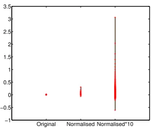
Original Normalised Normalised*10 −1

−0.5 0 0.5 1 1.5 2 2.5 3 3.5

Figure 1: The range of context weights on tTest weighted vectors before and after normalisation.

Context Ranking and Selection The weight-ing schemes change the importance of individ-ual target-context raw co-occurrence counts by considering the frequency with which each con-text word occurs with other target words. This is similar to term-weighting in IR and many re-trieval functions are also used as weighting func-tions in DSMs. In the retrieval-based model ESA (Gabrilovich and Markovitch, 2007), only theN highest-weighted contexts are kept as a represen-tative set of “topics” for a particular target word, and the rest are set to zero. Here we use a sim-ilar technique and, for each target word, retain only theN-highest weighted context words, using a word-similarity development set to choose the N that maximises correlation across all words in that dataset. Throughout the paper, we will refer to this technique as context selection (CS) and use N to indicate the maximum number of contexts per word. Hence all word vectors have at mostN non-zero elements, effectively adjusting the spar-sity of the vectors, which may have an effect on the sum and elementwise product operations when composing vectors.

Normalisation PPMI has only positive values that span the range r0,8s, while tTest spans

r1,1s, but generally produces values tightly con-centrated around zero. We found that these ranges can produce poor performance due to numerical problems, so we corrected this through weighted row normalisation: ~w:λ_||w~w~_||2. Withλ10this has the effect of restricting the values tor10,10s

for tTest andr0,10sfor PPMI. Figure 1 shows the range of values for tTest. In general we useλ1, but for some experiments we useλ 10to push the highest weights above 1, as a way of combat-ing the numerical errors that are likely to arise due

to repeated multiplications of small numbers. This normalisation has no effect on the ordering of con-text weights or cosine similarity calculations be-tween single-word vectors. We apply normalisa-tion prior to dimensionality reducnormalisa-tion and RI.

SVD SVD transforms vectors from their target-context representation into a target-topic space. The resulting space is dense, in that the vectors no longer contain any zero elements. If M is a

|w| |C|matrix whose rows are made of word vectorsw~i, then the lower dimensional representa-tion of those vectors is encoded in the|W| K matrix MˆK UKSK where SVDpM, Kq

UKSKVK (Deerwester et al., 1990). We also tried non-negative matrix factorisation (NNMF) (Seung and Lee, 2001), but found that it did not perform as well as SVD. We used the standard Matlab implementation of SVD.

Random Indexing There are two ways of creat-ing RI-based DSMs, the most popular becreat-ing to ini-tialise all target word vectors to zero and to gener-ate a random vector for each context word. Then, while traversing through the corpus, each time a target word and a context word co-occur, the con-text word vector is added to the vector represent-ing the target word. This method allows the RI vectors to be created in one step through a single traversal of the corpus. The other method, follow-ing Jones and Mewhort (2007), is to create the RI vectors through matrix multiplication rather than sequentially. We employ this method and assign each context word a random vector e~cj trkuk

whererk are drawn from the normal distribution

Np0, 1

Dq and|e~cj| D 4096. The RI

repre-sentation of a target wordRIpw~iq w~iRis con-structed by multiplying the word vector w~i, ob-tained as before, by the|C| DmatrixRwhere each column represents the vectorse~cj. Weighting

is performed prior to random indexing.

3 Word Similarity Experiments

tTest PPMI Freq Data Maxρ Fullρ Maxρ Fullρ Maxρ Fullρ

MENdev: 0.75 0.73 0.76 0.61 0.66 0.57

MENtest 0.76 0.73 0.76 0.61 0.66 0.56

WS353 0.70 0.63 0.70 0.41 0.57 0.41

Table 1: ValuesN learned on dev (:) also improve performance on the test data. Maxρindicates cor-relation at the values of N that lead to the high-est Spearman correlation on the development data. For each weighting scheme these are: 140 (tTest), 240 (PPMI), and 20 (Freq). Full ρ indicates the correlation when using full vectors without CS.

The cosine, Jaccard, and Lin similarity mea-sures (Curran, 2004) were all used to ensure the results reflect genuine effects of context selection, and not an artefact of any particular similarity measure. The similarity measure and value ofN were chosen, given a particular weighting scheme, to maximise correlation on the development part of the MEN data (Bruni et al., 2012) (MENdev). Testing was performed on the remaining section of MEN and the entire WS353 dataset (Finkelstein et al., 2002). The MEN dataset consists of 3,000 word pairs rated for similarity, which is divided into a 2,000-pair development set and a 1,000-pair test set. WS353 consists only of 353 pairs, but has been consistently used as a benchmark word simi-larity dataset throughout the past decade.

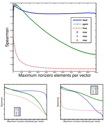
Results Figure 2 shows how correlation varies with N for the MEN development data. The peak performance for tTest is achieved when using around 140 top-ranked contexts per word, while for PPMI it is atN 240, and for FreqN 20. The dramatic drop in performance is demonstrated when using all three similarity measures, although Jaccard seems particularly sensitive to the nega-tive tTest weights that are introduced when lower-ranked contexts are added to the vectors. The re-maining experiments only consider cosine similar-ity. We also find that context selection improves correlation for tTest, PPMI, and the unweighted Freq vectors on the test data (Table 1). Moreover, the lower the correlation from the full vectors, the larger the improvement when using CS.

3.1 Dimensionality Reduction

Figure 3 shows the effects of dimensionality re-duction described in the following experiments.

0 1000 2000 3000 4000 5000 6000 7000 8000 9000 10000 0.58

0.6 0.62 0.64 0.66 0.68 0.7 0.72 0.74 0.76

Maximum nonzero elements per vector

Spearman

ttest

ppmi

freq

max

max

max

0 1000 2000 3000 4000 5000 6000 7000 8000 9000 10000 0.1

0.2 0.3 0.4 0.5 0.6 0.7 0.8

Maximum nonzero elements per vector

Spearman

ttest ppmi freq max max max

0 1000 2000 3000 4000 5000 6000 7000 8000 9000 10000 0

0.1 0.2 0.3 0.4 0.5 0.6 0.7 0.8

Maximum nonzero elements per vector

Spearman

ttest ppmi freq max max max

Figure 2: Correlation decreases as more lower-ranked context words are introduced (MENdev), with cosine (top), Lin (bottom left), and Jaccard (bottom right) simialrity measures.

3.1.1 SVD and CS

To check whether CS improves the correlation through increased sparsity or whether it improves the contextual representation of the words, we in-vestigated the behaviour of SVD on three differ-ent levels of vector sparsity. To construct the most sparse vectors, we chose the best performing N for each weighting scheme (from Table 1). Thus sparse tTest vectors had 140

10000 0.0140, or 1.4%,

non-zero elements. We also chose a mid-range of N 3300 for up to 33% of non-zero ele-ments per vector, and finally the full vectors with

N 10000.

Results In general the CS-tuned vectors lead to better lower-dimensional representations. The mid-range contexts in the tTest weighting scheme seem to hold information that hinders SVD, while the lowest-ranked negative weights appear to help (when the mid-range contexts are present as well). For the PPMI weighting, fewer contexts consis-tently lead to better representations, while the un-weighted vectors seem to mainly hold information in the top 20 most frequent contexts for each word.

3.1.2 SVD, CS, and Normalisation

0 100 200 300 400 500 600 700 800 0.3

0.4 0.5 0.6 0.7 0.8

Number of dimensions (K)

Spearman

tTest

140 N=3300 N=10000 norm 140 norm N=3300 norm N=10000 all 140 all N=3300 all N=10000

0 100 200 300 400 500 600 700 800 0.1

0.2 0.3 0.4 0.5 0.6 0.7 0.8

Number of dimensions (K)

Spearman

PPMI

240 N=3300 N=10000 norm 240 norm N=3300 norm N=10000 all 240 all N=3300 all N=10000

0 100 200 300 400 500 600 700 800 0.2

0.3 0.4 0.5 0.6 0.7

Number of dimensions (K)

Spearman

Freq

20 N=3300 N=10000 norm 20 norm N=3300 norm N=10000 all 20 all N=3300 all N=10000

Figure 3: Vectors tuned for sparseness (blue) consistently produce equal or better dimensionality reduc-tions (results on MENdev). The solid lines show improvement in lower dimensional representareduc-tions of SVD when dimensionality reduction is applied after normalisation.

Results Normalisation leads to more stable SVD representations, with a large improvement for small numbers of dimensions (K) as demonstrated by the solid lines in Figure 3. At K 20 the Spearman correlation increases from 0.61 to 0.71. In addition, for tTest there is an improvement in the mid-range vectors, and a knock-on effect for the full vectors. As the tTest values effectively range from0.1to0.1, the mid-range values are very small numbers closely grouped around zero. Normalisation spreads and increases these num-bers, perhaps making them more relevant to the SVD algorithm. The effect is also visible for PPMI weighting where atK 20the correlation increases from 0.48 to 0.70. For PPMI and Freq we also see that, for the full and mid-range vec-tors, the SVD representations have slightly higher correlations than the unreduced vectors.

3.2 Random Indexing

We use random indexing primarily to produce a vector representation for convolution (Section 4). While this produces a lower-dimensional repsentation, it may not use less memory since the re-sulting vectors, although smaller, are fully dense.

In summary, the RI encoded vectors with di-mensions of D 4096 lead to only slightly re-duced correlation values compared to their unen-coded counterparts. We find that for tTest we get similar performance with or without CS at any level, while for PPMI CS helps especially for D¥ 512. On Freq we find that CS withN 60

leads to higher correlation, but mid-range and full vectors have equivalent performance. For Freq, the correlation is equivalent to full vectors from D 128, while for the weighted vectors 512 di-mensions appear to be sufficient. Unlike for SVD, normalisation slightly reduces the performance for mid-range dimensions.

4 Compositional Experiments

We examine the performance of vectors aug-mented by CS and normalisation in two compo-sitional tasks. The first is an extension of the word similarity task to phrase pairs, using the dataset of Mitchell and Lapata (2010). Each entry in the dataset consists of two phrases, each consisting of two words (in various syntactic relations, such as verb-object and adjective noun), and a gold stan-dard score. We combine the two word vectors into a single phrase vector using various operators de-scribed below. We then calculate the similarity between the phrase vectors using cosine and com-pare the resulting scores against the gold standard using Spearman correlation. The second task is our new definitions task where, again, word vec-tors from each definition are composed to form a single vector, which can then be compared for sim-ilarity with the target term.

We use PPMI- and tTest-weighted vectors at three CS cutoff points: the best chosen N from Section 3, the top third of the ranked contexts at N 3300, and the full vectors without CS at

N 10000. This gives us a range of values to

examine, without directly tuning on this dataset. For dimensionality reduction we consider vectors reduced with SVD to 100 and 700 dimensions. In some cases we exclude the results for SVD700

be-cause they are very close to the scores for unre-duced vectors. We experiment with 3 values ofD fromt512,1024,4096ufor the RI vectors.

de-fined as follows for two word vectors~x, ~y:

Sum ~x ~y t~xi ~yiu_i

Prod ~xd~y t~xi~yiui

Kron ~xb~y t~xi~yju_ij

Conv ~xg~y!°n_j0p~xq_j%n p~yq_pijq%n)

i Repeated application of theSumoperation adds contexts for each of the words that occur in a phrase, which maintains (and mixes) any noisy parts of the component word vectors. Our inten-tion was that use of the CS vectors would lead to less noisy word vectors and hence less noisy phrase and sentence vectors. The Prodoperator, on the other hand, provides a phrase or sentence representation consisting only of the contexts that are common to all of the words in the sentence (since zeros in any of the word vectors lead to zeros in the same position in the sentence vec-tor). This effect is particularly problematic for rare words which may have sparse vectors, leading to a sparse vector for the sentence.1 _{We address the}

sparsity problem through the use of dimensional-ity reduction, which produces more dense vectors.

Kron, the Kronecker (or tensor) product of two vectors, produces a matrix (second order tensor) whose diagonal matches the result of the Prod

operation, but whose off-diagonal entries are all the other products of elements of the two vectors. We only applyKronto SVD-reduced vectors, and to compare two matrices we turn them into vec-tors by concatenating matrix rows, and use co-sine similarity on the resulting vectors. While in the more complex, type-driven methods (Baroni and Zamparelli, 2010; Coecke et al., 2010) ten-sors represent functions, and off-diagonal entries have a particular transformational interpretation as part of a linear map, the significance of the off-diagonal elements is difficult to interpret in our setting, apart from their role as encoders of the or-der of operands. We only examineKronas the un-encoded version of theConvoperator to see how the performance is affected by the random index-ing and the modular summation by which Conv

differs fromKron.2 _{We cannot useKronfor}

com-bining more than two words as the size of the re-sulting tensor grows exponentially with the

num-1_{Sparsity is a problem that may be addressable through}

smoothing (Zhai and Lafferty, 2001), although we do not in-vestigate that avenue in this paper.

2_{Convalso differs fromKronin that it is commutative,}

unless one of the operands is permuted. In this paper we do not permute the operands.

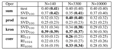
Oper N=140 N=3300 N=10000

sum ttest_SVD 0.40(0.41) 0.40 (0.40) 0.40 (0.40)

100 0.37(0.42) 0.35(0.41) 0.37 (0.40)

prod ttest_SVD 0.32 (0.32) 0.40 (0.40) 0.32 (0.32)

100 0.25 (0.23) 0.23 (0.23) 0.21 (0.23)

kron SVD100 0.31 (0.34) 0.34(0.38) 0.29 (0.32)

SVD700 0.39 (0.39) 0.37 (0.37) 0.30 (0.30)

conv RI512 0.10 (0.12) 0.26(0.21) 0.25 (0.25)

RI1024 0.22 (0.15) 0.29 (0.27) 0.25 (0.26)

RI4096 0.16 (0.19) 0.33 (0.34) 0.28 (0.30)

Table 2: Behaviour of vector operators with tTest vectors on ML2010 (Spearman correlation). Val-ues for normalised vectors in parentheses.

Oper N=240 N=3300 N=10000

sum ppmi_SVD 0.40(0.39) 0.40 (0.39) 0.29 (0.29)

100 0.40(0.40) 0.38(0.40) 0.29 (0.30)

prod ppmi_SVD 0.28 (0.28) 0.40 (0.40) 0.30 (0.30)

100 0.23 (0.17) 0.18 (0.22) 0.14 (0.12)

kron SVD100 0.37 (0.30) 0.36(0.38) 0.27 (0.27)

SVD700 0.38 (0.37) 0.37 (0.37) 0.26 (0.26)

conv RI512 0.09 (0.09) 0.27(0.30) 0.25 (0.24)

RI1024 0.08 (0.14) 0.33(0.37) 0.25 (0.27)

RI4096 0.18 (0.19) 0.37 (0.38) 0.27 (0.27)

Table 3: Behaviour of vector operators with PPMI vectors on ML2010 (Spearman correlation). Val-ues for normalised vectors in parentheses.

ber of vector operations, but we can useConvas an encoded alternative as it results in a vector of the same dimension as the two operands.

4.1 Phrase Similarity

To test how CS, normalisation, and dimensional-ity reduction affect simple compositional vector operations we use the test portion of the phrasal similarity dataset from Mitchell and Lapata (2010) (ML2010). This dataset consists of pairs of two-word phrases and a human similarity judgement on the scale of 1-7. There are three types of phrases: noun-noun, adjective-noun, and verb-object. In the original paper, and some subse-quent works, these were treated as three different datasets; however, here we combine the datasets into one single phrase pair dataset. This allows us to summarise the effects of different types of vec-tors on phrasal composition in general.

Results Our results (Tables 2 and 3) are compa-rable to those in Mitchell and Lapata (2010) av-eraged across the phrase-types (ρ 0.44), but are achieved with much smaller vectors. We find that with normalisation, and the optimal choice ofN, there is little difference betweenProd and

Sum. Sum and Kron benefit from normalisa-tion, especially in combination with SVD, but for

Conv) have a preference for context selection that includes the mid-rank contexts (N 3300), but not the full vector (N 10000). On tTest vec-tors Sum is relatively stable across different CS and SVD settings, but with PPMI weighting, there is a preference for lowerN. SVD reduces perfor-mance forProd, but not forKron. Finally,Conv

gets higher correlation with higher-dimensional RI vectors and with PPMI weights.

4.2 Definition Retrieval

In this task, which is formulated as a retrieval task, we investigate the behaviour of different vector operators as multiple operations are chained to-gether. We first encode each definition into a sin-gle vector through repeated application of one of the operators on the distributional vectors of the content words in the definition. Then, for each head (defined) word, we rank all the different defi-nition vectors in decreasing order according to in-ner product (unnormalised cosine) similarity with the head word’s distributional vector.

Performance is measured using precision and Mean Reciprocal Rank (MRR). If the correct defi-nition is ranked first, the precision (P@1) is 1, oth-erwise 0. Since there is only one definition per head word, the reciprocal rank (RR) is the inverse of the rank of the correct definition. So if the cor-rect definition is ranked fourth, for example, then RR is 1₄. MRR is the average of the RR across all head words.

The difficulty of the task depends on how many words there are in the dataset and how similar their definitions are. In addition, if a head word oc-curs in the definition of another word in the same dataset, it may cause the incorrect definition to be ranked higher than the correct one. These prob-lems are more likely to occur with higher fre-quency words and in a larger dataset. In order to counter these effects, we average our results over ten repeated random samplings of 100 word-definition pairs. The sampling also gives us a ran-dombaselinefor P@1 of0.01300.0106and for MRR0.05760.0170, which can be interpreted as there is a chance of slightly more than 1 in 100 of ranking the correct definition first, and on aver-age the correct definition is ranked around the 20 mark.

For this task all experiments were performed using the tTest-weighted vectors. When applying normalisation we useλ 1(Norm) andλ 10

DD2 DD3 DD4 DD5 DD6 DD7 DD8 DD9 DD10

346 547 594 537 409 300 216 150 287

Table 4: Number of definitions per dataset.

(Norm10). In addition, we examine the effect of continually applyingNorm after every operation (CNorm).

Dataset We developed a new dataset (DD) con-sisting of 3,386 definitions from the Wiktionary BNC spoken-word frequency list.3 _{Most of the}

words have several definitions, but we considered only the first definition with at least two non-stopwords. The word-definition pairs were di-vided into nine separate datasets according to the number of non-stopwords in the definition. For ex-ample, all of the definitions that have five content words are inDD5. The exception isDD10, which contains all the definitions of ten or more words. Table 4 shows the number of definitions in each dataset.

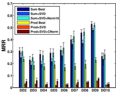
Results Figure 4 shows how the MRR varies with different DD datasets for Sum, Prod, and

Conv. The CS, SVD, and RI settings for each op-erator correspond to the best average settings from Table 5. In some cases other settings had simi-lar performance, but we chose these for illustrative purposes. We can see that all operators have rel-atively higher MRR on smaller datasets (DD6-9). Compensating for that effect, we can hypothesise thatSumhas a steady performance across differ-ent definition sizes, while the performance of both

Prod and Convdeclines as the number of oper-ations increases. Normalisation helps withSum

throughout, with little difference in performance betweenNormandNorm10, but with a slight de-crease whenCNormis used. On the other hand, onlyCNormimproves the ranking ofProd-based vectors. Normalisation makes no difference for RI vectors combined with convolution and the results in Table 5 show that, on average, Convperforms worse than the random baseline.

In Figure 5 we can see that, although dimen-sionality reduction leads to lower MRR, forSum, normalisation prior to SVD counteracts this effect, while, forProd, dimensionality reduction, in gen-eral, reduces the performance.

DD2 DD3 DD4 DD5 DD6 DD7 DD8 DD9 DD10 0

0.1 0.2 0.3 0.4 0.5 0.6 0.7

MRR

Sum Sum+Norm Prod Prod+Norm Conv Conv+Norm DDsize/1000

Figure 4: Per-dataset breakdown of best nor-malised and unnornor-malised vectors for each vector operator. Stars indicate the dataset size from Ta-ble 4 divided by 1000.

Sum Prod Conv

Norm No Yes No CN No Yes

CS (N) 140 140 3300 10000 140 3300

SVD(K)/RI(D) 700 700 None None 2048 512

mean P@1 0.18 0.23 0.01 0.11 0.00 0.00

mean MRR 0.28 0.35 0.06 0.17 0.02 0.02

Table 5: Best settings for operators calculated from the highest average MRR across all the datasets, with and without normalisation. The results for vectors with no normalisation or CS are: Sum - P@1=0.1567, MRR=0.2624; Prod -P@1=0.0147, MRR=0.0542;ConvP@1=0.0027, MRR=0.0192.

5 Discussion

In this paper we introduced context selection and normalisation as techniques for improving the se-mantic vector space representations of words. We found that, although our untuned vectors perform better on WS353 data (ρ0.63) than vectors used by Mitchell and Lapata (2010) (ρ 0.42), our best phrase composition model (Sum, ρ 0.40) produces a lower performance than an estimate of their best model (Prod,ρ0.44).4_{This indicates}

that better performance on word-similarity data does not directly translate into better performance on compositional tasks; however, CS and normal-isation are both effective in increasing the qual-ity of the composed representation (ρ 0.42). Since CS and normalisation are computationally inexpensive, they are an excellent way to improve model quality compared to the alternative, which

4_{The estimate is computed as an average across the three}

phrase-type results.

DD2 DD3 DD4 DD5 DD6 DD7 DD8 DD9 DD10 0

0.1 0.2 0.3 0.4 0.5 0.6 0.7

MRR

Sum Best

Sum+SVD

Sum+SVD+Norm10

Prod Best

Prod+SVD

Prod+SVD+CNorm

Figure 5: Per-dataset breakdown of best nor-malised and unnornor-malised SVD vectors forSum

andProd. For both operators the best CS and SVD settings for normalised vectors were N 140, K 700, and for unnormalised wereN 10000, K 700.

is building several models with various context types, in order to find which one suits the data best. Furthermore, we show that, as the number of vector operations increases, Sumis the most sta-ble operator and that it benefits from sparser rep-resentations (lowN) and normalisation. Employ-ing both of these methods, we are able to build an SVD-based representation that performs as well as full-dimensional vectors which, together with

Sum, give the best results on both phrase and def-inition tasks. In fact, normalisation and CS both improve the SVD representations of the vectors across different weighting schemes. This is a key result, as many of the more complex composi-tional methods require low dimensional represen-tations for computational reasons.

Future work will include application of CS and normalised lower-dimensional vectors to more complex compositional methods, and investiga-tions into whether these strategies apply to other context types and other dimensionality reduction methods such as LDA (Blei et al., 2003).

Acknowledgements

References

Jacob Andreas and Zoubin Ghahramani. 2013. A gen-erative model of vector space semantics. In Pro-ceedings of the ACL 2013 Workshop on Continu-ous Vector Space Models and their Compositional-ity, Sofia, Bulgaria.

M. Baroni and R. Zamparelli. 2010. Nouns

are vectors, adjectives are matrices: Representing adjective-noun constructions in semantic space. In

Conference on Empirical Methods in Natural Lan-guage Processing (EMNLP-10), Cambridge, MA. David M. Blei, Andrew Y. Ng, and Michael I. Jordan.

2003. Latent dirichlet allocation. J. Mach. Learn. Res., 3:993–1022.

Elia Bruni, Gemma Boleda, Marco Baroni, and Nam Khanh Tran. 2012. Distributional semantics in technicolor. In Proceedings of the 50th Annual Meeting of the Association for Computational Lin-guistics (Volume 1: Long Papers), pages 136–145, Jeju Island, Korea, July. Association for Computa-tional Linguistics.

Daoud Clarke. 2012. A context-theoretic frame-work for compositionality in distributional seman-tics. Comput. Linguist., 38(1):41–71, March. B. Coecke, M. Sadrzadeh, and S. Clark. 2010.

Math-ematical foundations for a compositional distribu-tional model of meaning. In J. van Bentham, M. Moortgat, and W. Buszkowski, editors, Linguis-tic Analysis (Lambek Festschrift), volume 36, pages 345–384.

James R. Curran. 2004. From Distributional to Seman-tic Similarity. Ph.D. thesis, University of Edinburgh. Scott Deerwester, Susan T. Dumais, Thomas K. Lan-dauer, George W. Furnas, and Richard Harshman. 1990. Indexing by latent semantic analysis.Journal of the Society for Information Science, 41(6):391– 407.

Lev Finkelstein, Evgeniy Gabrilovich, Yossi Matias, Ehud Rivlin, Zach Solan, Gadi Wolfman, and Ey-tan Ruppin. 2002. Placing search in context: The concept revisited. ACM Transactions on Informa-tion Systems, 20:116–131.

Evgeniy Gabrilovich and Shaul Markovitch. 2007. Computing semantic relatedness using Wikipedia-based explicit semantic analysis. InProceedings of the 20th international joint conference on Artifical intelligence, IJCAI’07, pages 1606–1611, San Fran-cisco, CA, USA. Morgan Kaufmann Publishers Inc. Pablo Gamallo and Stefan Bordag. 2011. Is singu-lar value decomposition useful for word simisingu-larity extraction? Language Resources and Evaluation, 45(2):95–119.

Michael N. Jones and Douglas J. K. Mewhort. 2007. Representing word meaning and order information

in a composite holographic lexicon. Psychological Review, 114:1–37.

Ekaterina Kochmar and Ted Briscoe. 2013. Capturing anomalies in the choice of content words in compo-sitional distributional semantic space. In Proceed-ings of the Recent Advances in Natural Language Processing (RANLP-2013), Hissar, Bulgaria. Guido Minnen, John Carroll, and Darren Pearce. 2001.

Applied morphological processing of English. Nat-ural Language Engineering, 7(3):207–223.

Jeff Mitchell and Mirella Lapata. 2010. Composition in distributional models of semantics. Cognitive Sci-ence, 34(8):1388–1429.

T. A. Plate. 1991. Holographic reduced Repre-sentations: Convolution algebra for compositional distributed representations. In J. Mylopoulos and R. Reiter, editors, Proceedings of the 12th Inter-national Joint Conference on Artificial Intelligence, Sydney, Australia, August 1991, pages 30–35, San Mateo, CA. Morgan Kauffman.

D Seung and L Lee. 2001. Algorithms for non-negative matrix factorization. Advances in neural information processing systems, 13:556–562. Richard Socher, Brody Huval, Christopher D.

Man-ning, and Andrew Y. Ng. 2012. Semantic Composi-tionality Through Recursive Matrix-Vector Spaces. In Proceedings of the 2012 Conference on Em-pirical Methods in Natural Language Processing (EMNLP), Jeju Island, Korea.

Peter Turney and Patrick Pantel. 2010. From fre-quency to meaning: Vector space models of se-mantics. Journal of Artificial Intelligence Research, 37:141–188.

Fabio Massimo Zanzotto and Lorenzo Dell’Arciprete. 2011. Distributed structures and distributional meaning. InProceedings of the Workshop on Dis-tributional Semantics and Compositionality, DiSCo-11, pages 10–15, Portland, Oregon. Association for Computational Linguistics.