Posing Fair Generalization Tasks for Natural Language Inference

Proceedings of the 2019 Conference on Empirical Methods in Natural Language Processing 4485

Posing Fair Generalization Tasks for Natural Language Inference

Atticus Geiger

Stanford Symbolic Systems Program

[email protected]

Lauri Karttunen

Stanford Linguistics

[email protected]

Ignacio Cases

Stanford Linguistics

[email protected]

Christopher Potts

Stanford Linguistics

[email protected]

Abstract

Deep learning models for semantics are gener-ally evaluated using naturalistic corpora. Ad-versarial methods, in which models are eval-uated on new examples with known semantic properties, have begun to reveal that good per-formance at these naturalistic tasks can hide serious shortcomings. However, we should in-sist that these evaluations be fair – that the models are given data sufficient to support the requisite kinds of generalization. In this pa-per, we define and motivate a formal notion of fairness in this sense. We then apply these ideas to natural language inference by con-structing very challenging but provably fair ar-tificial datasets and showing that standard neu-ral models fail to geneneu-ralize in the required ways; only task-specific models that jointly compose the premise and hypothesis are able to achieve high performance, and even these models do not solve the task perfectly.

1 Introduction

Evaluations of deep learning approaches to seman-tics generally rely on corpora of naturalistic exam-ples, with quantitative metrics serving as a proxy for the underlying capacity of the models to learn rich meaning representations and find generalized solutions. From this perspective, when a model achieves human-level performance on a task ac-cording to a chosen metric, one might be tempted to say that the task is “solved”. However, recent adversarial testing methods, in which models are evaluated on new examples with known semantic properties, have begun to reveal that even these state-of-the-art models often rely on brittle, local solutions that fail to generalize even to examples that are similar to those they saw in training. These findings indicate that we need a broad and deep range of evaluation methods to fully characterize the capacities of our models.

However, for any evaluation method, we should ask whether it isfair. Has the model been shown data sufficient to support the kind of generaliza-tion we are asking of it? Unless we can say “yes” with complete certainty, we can’t be sure whether a failed evaluation traces to a model limitation or a data limitation that no model could overcome.

In this paper, we seek to address this issue by defining a formal notion of fairness for these eval-uations. The definition is quite general and can be used to create fair evaluations for a wide range of tasks. We apply it to Natural Language Infer-ence (NLI) by constructing very challenging but provably fair artificial datasets. We evaluate a number of different standard architectures (vari-ants of LSTM sequence models with attention and tree-structured neural networks) as well as NLI-specific tree-structured neural networks that pro-cess aligned examples. Our central finding is that only task-specific models are able to achieve high performance, and even these models do not solve the task perfectly, calling into question the viabil-ity of the standard models for semantics.

2 Related Work

There is a growing literature that uses targeted generalization tasks to probe the capacity of learn-ing models. We seek to build on this work by de-veloping a formal framework in which one can ask whether one of these tasks is even possible.

In adversarial testing, training examples are sys-tematically perturbed and then used for testing. In computer vision, it is common to adversari-ally train on artificiadversari-ally noisy examples to create a more robust model (Goodfellow et al., 2015;

need for models with stronger generalization ca-pabilities. Similarly, adversarial testing has shown that strong models for the SNLI dataset ( Bow-man et al., 2015a) have significant holes in their knowledge of lexical and compositional semantics (Glockner et al.,2018;Naik et al.,2018;Nie et al.,

2018;Yanaka et al.,2019;Dasgupta et al.,2018). In addition, a number of recent papers suggest that even top models exploit dataset artifacts to achieve good quantitative results (Poliak et al.,2018; Gu-rurangan et al.,2018;Tsuchiya,2018), which fur-ther emphasizes the need to go beyond naturalistic evaluations.

Artificially generated datasets have also been used extensively to gain analytic insights into what models are learning. These methods have the ad-vantage that the complexity of individual exam-ples can be precisely characterized without refer-ence to the models being evaluated. Evans et al.

(2018) assess the ability of neural models to learn propositional logic entailment. Bowman et al.

(2015b) conduct similar experiments using natu-ral logic, andVeldhoen and Zuidema(2018) ana-lyze models trained on those same tasks, arguing that they fail to discover the kind of global solu-tion we would expect if they had truly learned nat-ural logic. Lake and Baroni(2017) apply similar methods to instruction following with an artificial language describing a simple domain.

These methods can provide powerful insights, but the issue of fairness looms large. For in-stance,Bowman(2013) poses generalization tasks in which entire reasoning patterns are held out for testing. Similarly,Veldhoen and Zuidema(2018) assess a model’s ability to recognize De Morgan’s laws without any exposure to this reasoning in training. These extremely difficult tasks break from standard evaluations in an attempt to expose model limitations. However, these tasks are not fair by our standards; brief formal arguments for these claims are given in AppendixA.

3 Compositionality and Generalization

Many problems can be solved by recursively com-posing intermediate representations with functions along a tree structure. In the case of arithmetic, the intermediate representations are numbers and the functions are operators such a plus or minus. In the case of evaluating the truth of propositional logic sentences, the intermediate representation are truth values and the functions are logical

op-Data:A composition treeC= (T,Dom,Func), a node

a∈NT_{, and an inputx∈ I} C

Result:An output fromDom(a) functioncompose(C, a, x)

ifa∈NT leafthen

i←index(a, T) returnxi

else

c1, . . . cm←children(a, T)

returnFunc(a)(

compose(C, c1, x), . . . , compose(C, cm, x))

end

Algorithm 1: Recursive composition up a tree. This algorithm uses helper functions

children(a, T), which returns the left-to-right ordered children of node a, and index(a, T), which returns the index of a leaf according to left-to-right ordering.

erators such as disjunction, negation, or the ma-terial conditional. We will soon see that, in the case of NLI, the intermediate representations are semantic relations between phrases and the func-tions are semantic operators such as quantifiers or negation. When tasked with learning some com-positional problem, we intuitively would expect to be shown how every function operates on ev-ery intermediate value. Otherwise, some functions would be underdetermined. We now formalize the idea of recursive tree-structured composition and this intuitive notion of fairness.

We first define composition trees (Section3.1) and show how these naturally determine baseline learning models (Section3.2). These models im-plicitly define a property of fairness: a train/test split is fair if the baseline model learns the task perfectly (Section3.3). This enables us to create provably fair NLI tasks in Section4.

3.1 Composition Trees

A composition tree describes how to recursively compose elements from an input space up a tree structure to produce an element in an output space. Our baseline learning model will construct a com-position tree using training data.

Definition 1. (Composition Tree) LetT be an or-dered tree with nodes NT = N_leafT ∪N_non-leafT , where N_leafT is the set of leaf nodes and N_non-leafT

Data:An ordered treeT and a set of training dataD

containing pairs(x, Y)wherexis an input and

Y is a function defined onNT

non-leafproviding labels at every node ofT.

Result:A composition tree(T,Dom,Func) functionlearn(T,D)

Dom,Func←initialize(T) for(x, Y)∈ Ddo

Dom,Func←

memorize(x, Y, T,Dom,Func, r) end

return(T,Dom,Func)

functionmemorize(x,Y,T,Dom,Func,a) ifa∈NleafT then

i←index(a, T) Dom[a]←Dom[a]∪ {xi}

returnDom,Func else

Dom[a]←Dom[a]∪ {Y(a)} c1, . . . , cm←children(a, T)

Func[a][(Y(c1), . . . , Y(cm))]←Y(a)

fork←1. . . mdo Dom,Func←

memorize(x, Y, T,Dom,Func, ck)

end

returnDom,Func end

Algorithm 2:Given a tree and training data with labels for every node of the tree, this learning model constructs a composition tree. This al-gorithm uses helper functionschildren(a, T) andindex(a, T), as in Algorithm1, as well as

initialize(T), which returnsDom, a dictio-nary mappingNT to empty sets, andFunc, a dic-tionary mappingN_non-leafT to empty dictionaries.

N_non-leafT that assigns a function to each non-leaf node satisfying the following property: For any

a ∈ N_non-leafT with left-to-right ordered children

c1, . . . , cm, we have that Func(a) : Dom(c1) × · · · ×Dom(cm)→Dom(a). We refer to the tuple

C = (T,Dom,Func) as acomposition tree. The input spaceof this composition tree is the carte-sian product IC = Dom(l1) × · · · × Dom(lk),

wherel1, . . . , lk are the leaf nodes in left-to-right

order, and the output space is OC = Dom(r)

whereris the root node.

A composition tree C = (T,Dom,Func) re-alizes a function F : I_C → O_C in the follow-ing way: For any input x ∈ IC, this function is

given by F(x) = compose(C, r, x), wherer is the root node of T andcompose is defined re-cursively in Algorithm 1. For a given x ∈ IC

anda∈N_non-leafT with childrenc1, . . . , cm, we say

that the element of Dom(c1) × · · · × Dom(cm)

that is input to Func(a) during the computation of F(x) = compose(C, r, x) is the input real-ized atFunc(a)on xand the element ofDom(a) that is output byFunc(a)is the output realized at Func(a)onx. At a high level,compose(C, a, x) finds the output realized at a nodeaby computing nodea’s function Func(a) with the outputs real-ized at nodea’s children as inputs. This recursion bottoms out when the components of x are pro-vided as the outputs realized at leaf nodes.

3.2 A Baseline Learning Model

Algorithm 2 is our baseline learning model. It learns a function by constructing a composition tree. This is equivalent to learning the function that tree realizes, as once the composition tree is created, Algorithm1computes the realized func-tion. Because this model constructs a composition tree, it has an inductive bias to recursively com-pute intermediate representations up a tree struc-ture. At a high level, it constructs a full composi-tion tree when provided with the tree structure and training data that provides a label at every node in the tree by looping through training data inputs and memorizing the output realized at each inter-mediate function for a given input. As such, any learning model we compare to this baseline model should be provided with the outputs realized at ev-ery node during training.

3.3 Fairness

We define a training dataset to be fair with respect to some functionF if our baseline model perfectly learns the functionF from that training data. The guiding idea behind fairness is that the training data must expose every intermediate function of a composition tree to every possible intermediate in-put, allowing the baseline model to learn a global solution:

Definition 2. (A Property Sufficient for Fairness) A property of a training dataset D and tree T

that is sufficient for fairness with respect to a functionF is that there exists a composition tree

C = (T,Dom,Func) realizing F such that, for anya ∈ N_non-leafT and for any inputitoFunc(a), there exists(x, Y) ∈ Dwhereiis the input real-ized atFunc(a)onx.

de-C2→ {T,F}

C1 → {T,F}

{T,F} {¬, ε}

{⇒} {T,F}

Figure 1: A composition tree that realizes a function evaluating propositional sentences. We define the func-tionsC1(U, V1) =U(V1)andC2(V1,⇒, V2) =V1⇒

V2whereV1, V2∈ {T,F}andU ∈ {¬, ε}.

Train Test

T ⇒ εF T ⇒ ¬T

T ⇒ ¬F T ⇒ εT

F ⇒ ¬T F ⇒ ¬F

F ⇒ εT F ⇒ εF

Table 1: A fair train/test split for the evaluation prob-lem defined by the composition tree in Figure1. We give just the terminal nodes; the examples are full trees.

fine a challenging task, it is guaranteed to be pos-sible. We noted in Section2that some challenging problems in the literature fail to meet this minimal requirement.

3.4 Fair Tasks for Propositional Evaluation

As a simple illustration of the above concepts, we consider the task of evaluating the truth of a sen-tence from propositional logic. We use the stan-dard logical operators material conditional, ⇒, and negation, ¬, as well as the unary operator ε, which we define to be the identity function on

{T,F}. We consider a small set of eight propo-sitional sentences, all which can be seen in Ta-ble 1. We illustrate a composition tree that re-alizes a function performing truth evaluation on these sentences in Figure 1, where a leaf node l

is labeled with its domainDom(l) and a non-leaf nodeais labeled withFunc(a)→Dom(a).

A dataset for this problem is fair if and only if it has two specific properties. First, the binary operator ⇒ must be exposed to all four inputs in {T,F} × {T,F} during training. Second, the unary operators¬andεeach must be exposed to both inputs in{T,F}. Jointly, these constraints en-sure that a model will see all the possibilities for how our logical operators interact with their truth-value arguments. If either constraint is not met, then there is ambiguity about which operators the model is tasked with learning. An example fair

symbol example set theoretic definition

x≡y couch≡sofa x=y

x@y crow@bird x⊂y

xAy birdAcrow x⊃y

x∧y human ∧ nonhuman x∩y=∅ ∧x∪y=U x|y cat|dog x∩y=∅ ∧x∪y6=U x ^ y animal^nonhuman x∩y6=∅ ∧x∪y=U x#y hungry#hippo (all other cases) Table 2: The seven basic semantic relations of Mac-Cartney and Manning(2009):B={#= independence,

@= entailment,_A= reverse entailment,|= alternation,

^= cover,∧= negation,≡= equivalence}.

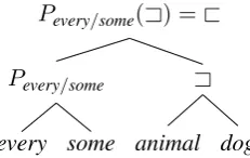
Pevery/some(A) =@

A

dog animal

Pevery/some

some every

Figure 2: Natural logic inference cast as composition on aligned semantic parse trees. The joint projectiv-ity signaturePevery/some operates on the semantic

rela-tion _Adetermined by the aligned pair animal/dog to determine entailment (_@) for the whole. In contrast, if we reverseeveryandsome, creating the examplesome animal/every dog, then the joint projectivity signature

Psome/everyoperates onA, which determines reverse

en-tailment (_A).

train/test split is given in Table1.

Crucial to our ability to create a fair training dataset using only four of the eight sentences is that⇒operates on the intermediate representation of a truth value, abstracting away from the specific identity of its sentence arguments. Because there are two ways to realize T and F at the intermedi-ate node, we can efficiently use only half of our sentences to satisfy our fairness property.

4 Fair Artificial NLI Datasets

Our central empirical question is whether current neural models can learn to do robust natural lan-guage inference if given fair datasets. We now present a method for addressing this question. To do this, we need to move beyond the simple propo-sitional logic example explored above, to come closer to the true complexity of natural language. To do this, we adopt a variant of thenatural logic developed by MacCartney and Manning (2007,

is a flexible approach to doing logical inference directly on natural language expressions. Thus, in this setting, we can work directly with natural lan-guage sentences while retaining complete control over all aspects of the generated dataset.

4.1 Natural Logic

We define natural logic reasoning over aligned se-mantic parse trees that represent both the premise and hypothesis as a single structure and allow us to calculate semantic relations for all phrases compo-sitionally. The core components aresemantic rela-tions, which capture the direct inferential relation-ships between words and phrases, andprojectivity signatures, which encode how semantic operators interact compositionally with their arguments. We employ the semantic relations ofMacCartney and Manning(2009), as in Table2. We useBto denote the set containing these seven semantic relations.

The essential concept for the material to come is that ofjoint projectivity: for a pair of semantic functions f and g and a pair of inputsX andY

that are in relationR, the joint projectivity signa-tureP_{f /g}:B → Bis a function such that the rela-tion betweenf(X)andg(Y)isPf /g(R). Figure2

illustrates this with the phrasesevery animal and some dog. We show the details of how the natural logic ofMacCartney and Manning(2009), with a small extension, determines the joint projectivity signatures for our datasets in AppendixB.

4.2 A Fragment of Natural Language

Our fragmentGconsists of sentences of the form:

QSAdjSNSNeg Adv V QOAdjONO

where NSand NOare nouns, V is a verb, AdjSand

Adj_Oare adjectives, and Adv is an adverb. Neg is does not, and Q_Sand Q_Ocan beevery,not every, some, orno; in each of the remaining categories, there are 100 words. Additionally, Adj_S, Adj_O, Adv, and Neg can be the empty string ε, which is represented in the data by a unique token. Se-mantic scope is fixed by surface order, with earlier elements scoping over later ones.

For NLI, we define the set of premise– hypothesis pairsS ⊂G×Gsuch that(sp, sh)∈ S

iff the non-identical non-empty nouns, adjectives, verbs, and adverbs with identical positions in sp

and sh are in the #relation. This constraint on S trivializes the task of determining the lexical relations between adjectives, nouns, adverbs, and verbs, since the relation is≡where the two aligned

elements are identical and otherwise#. Further-more, it follows that distinguishing contradictions from entailments is trivial. The only sources of contradictions are negation and the negative quan-tifiersnoandnot every. Consider(sp, sh)∈ Sand

letCbe the number of times negation or a negative quantifier occurs inspandsh. Ifspcontradictssh,

thenCis odd; ifspentailssh, thenCis even.

We constrain the open-domain vocabulary to stress models with learning interactions between logically complex function words; we trivialize the task of lexical semantics to isolate the task of compositional semantics. We also do not have multiple morphological forms, use artificial tokens that do not correspond to English words, and col-lapsedo notandnot everyto single tokens to fur-ther simplify the task and isolate a model’s ability to perform compositional logical reasoning.

Our corpora use the three-way labeling scheme of entailment, contradiction, and neutral. To assign these labels, we translate each premise– hypothesis pair into first-order logic and use Prover9 (McCune,2005–2010). We assume no ex-pression is empty or universal and encode these as-sumptions as additional premises. This label gen-eration process implicitly assumes the relation be-tween unequal nouns, verbs, adjectives, and ad-verbs is independence.

When we generate training data for NLI cor-pora from some subsetStrain ⊂ S, we perform the

following balancing. For a given example, every adjective–noun and adverb–verb pair across the premise and hypothesis is equally likely to have the relation ≡, @, A, or #. Without this bal-ancing, any given adjective–noun and adverb–verb pair across the premise and hypothesis has more than a 99% chance of being in the independence relation for values ofStrainwe consider. Even with

this step, 98% of the sentence pairs are neutral, so we again sample to create corpora that are bal-anced across the three NLI labels. This balancing across our three NLI labels justifies our use of an accuracy metric rather than an F1 score.

4.3 Composition Trees for NLI

We provide a composition tree for inference onS

COMP→ {≡,@,A,|,ˆ, ^,#}

COMP→ {≡,@,A,|,ˆ, ^,#}

COMP→ {≡,@,A,|,ˆ, ^,#}

COMP→ {#,@,A,≡} {#,≡}

NH O NP

O

PROJ→ A

AdjH O AdjP

O

PROJ→ Q

QH QP

COMP→ {#,@,A,≡} REL→ {#,≡}

VH VP

PROJ→ A

AdvH AdvP

PROJ→ N

N egH N egP

COMP→ {#,@,A,≡} REL→ {#,≡}

NH O NP

O

PROJ→ A

AdjH S AdjP

S

PROJ→ Q

QH QP

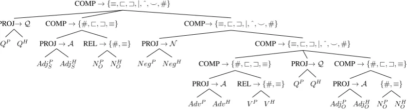
Figure 3: An aligned composition tree for inference on our set of examplesS. The superscriptsPandHrefer to premise and hypothesis. The semantic relations are defined in Table2. The setQis{some,every,no,not,every}. The setNegis{ε,not}. Qis the set of 16 joint projectivity signatures between the elements ofQ. N is the set of 4 joint projectivity signatures betweenεandno. Ais the set of 4 joint projectivity signatures betweenεand an intersective adjective or adverb. REL computes the semantic relations between lexical items, PROJ computes the joint projectivity between two semantic functions (Section4.1and AppendixB), and COMP applies semantic relations to joint projectivity signatures. This composition tree defines over1026distinct examples.

from the hypothesis. If both leaf nodes in a sibling pair have domains containing lexical items that are semantic functions, then their parent node domain contains the joint projectivity signatures between those semantic functions. Otherwise the parent node domain contains the semantic relations be-tween the lexical items in the two sibling node domains. The root captures the overall semantic relation between the premise and the hypothesis, while the remaining non-leaf nodes represent in-termediate phrasal relations.

The setsAdj_S,NS,AdjO,NO,Adv, andV each

have 100 of their respective open class lexical items with Adv, Adj_S, and Adj_O also containing the empty stringε. The setQis{some,every,no, not, every} and the setNeg is{ε,not}. Q is the set of 16 joint projectivity signatures between the quantifiers some, every, no, and not every, N is the set of 4 joint projectivity signatures between the empty string εandno, andA is the set of 4 projectivity signatures betweenεand an intersec-tive adjecintersec-tive or adverb. These joint projectivity signatures were exhaustively determined by us by hand, using the projectivity signatures of negation and quantifiers provided byMacCartney and Man-ning(2009) as well as a small extension (details in AppendixB).

The function PROJ computes the joint projec-tivity signature between two semantic functions, REL computes the semantic relation between two lexical items, and COMP inputs semantic relations into a joint projectivity signature and outputs the result. We trimmed the domain of every node so that the function of every node is surjective. Pairs

of subexpressions containing quantifiers can be in any of the seven basic semantic relations; even with the contributions of open-class lexical items trivialized, the level of complexity remains high, and all of it emerges from semantic composition, rather than from lexical relations.

4.4 A Difficult But Fair NLI Task

A fair training dataset exposes each local function to all possible inputs. Thus, a fair training dataset for NLI will have the following properties. First, all lexical semantic relations must be included in the training data, else the lexical targets could be underdetermined. Second, for any aligned seman-tic functionsf andgwith unknown joint projec-tivity signaturePf /g, and for any semantic relation

R, there is some training example wherePf /g is

exposed to the semantic relationR. This ensures that the model has enough information to learn full joint projectivity signatures. Even with these constraints in place, the composition tree of Sec-tion 3.1determines an enormous number of very challenging train/test splits. AppendixCfully de-fines the procedure for data generation.

We also experimentally verify that our baseline learns a perfect solution from the data we gener-ate. The training set contains 500,000 examples randomly sampled fromStrainand the test and

de-velopment sets each contain 10,000 distinct exam-ples randomly sampled from S¯train. All random

5 Models

We consider six different model architectures:

CBoW Premise and hypothesis are represented by the average of their respective word em-beddings (continuous bag of words).

LSTM Encoder Premise and hypothesis are pro-cessed as sequences of words using a recur-rent neural network (RNN) with LSTM cells, and the final hidden state of each serves as its representation (Hochreiter and Schmidhuber,

1997;Elman,1990;Bowman et al.,2015a).

TreeNN Premise and hypothesis are processed as trees, and the semantic composition func-tion is a single-layer feed-forward network (Socher et al.,2011b,a). The value of the root node is the semantic representation in each case.

Attention LSTM An LSTM RNN with word-by-word attention (Rockt¨aschel et al.,2015).

CompTreeNN Premise and hypothesis are pro-cessed as a single aligned tree, following the structure of the composition tree in Fig-ure3. The semantic composition function is a single-layer feed-forward network (Socher et al., 2011b,a). The value of the root node is the semantic representation of the premise and hypothesis together.

CompTreeNTN Identical to the CompTreeNN, but with a neural tensor network as the com-position function (Socher et al.,2013).

For the first three models, the premise and hy-pothesis representations are concatenated. For the CompTreeNN, CompTreeNTN, and Attention LSTM, there is just a single representation of the pair. In all cases, the premise–hypothesis repre-sentation is fed through two hidden layers and a softmax layer.

All models are initialized with random 100-dimensional word vectors and optimized us-ing Adam (Kingma and Ba, 2014). It would not be possible to use pretrained word vec-tors, due to the artificial nature of our dataset. A grid hyperparameter search was run over dropout values of {0,0.1,0.2,0.3} on the output and keep layers of LSTM cells, learning rates of{1e−2,3e−3,1e−3,3e−4}, L2 regularization values of {0,1e−4,1e−3,1e−2} on all weights, and activation functions ReLU and tanh. Each

sentence adverb-verb phrase

every tall kidhappily kicks everyrock happily kicks

entailment @

no tall kid does notkicks some large rock kicks negated verb phrases adjective-noun phrase happily kicks everyrock tall kid

| ≡

does notkicks some large rock tall kid

verb phrases single words

happily kicks everyrock tall≡tall

@ kid≡kid

kicks some large rock happily@ adjective-noun phrase single words

rock kicks≡kicks

A _Alarge

large rock rock≡rock

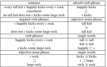
Figure 4: For any example sentence pair (top left) the neural models are trained using the a weighted sum of the error on 12 prediction tasks shown above. The 12 errors are weighted to regularize the loss according to the length of the expressions being predicted on.

hyperparameter setting was run for three epochs and parameters with the highest development set score were used for the complete training runs.

The training datasets for this generalization task are only fair if the outputs realized at every non-leaf node are provided during training just as they are in our baseline learning model. For our neu-ral models, we accomplish this by predicting se-mantic relations for every subexpression pair in the scope of a node in the tree in Figure 3 and summing the loss of the predictions together. We do not do this for the nodes labeled PROJ→ Q

or PROJ→ N, as the function PROJ is a bijec-tion at these nodes and no intermediate represen-tations are created. For any example sentence pair the neural models are trained using the a weighted sum of the error on 12 prediction tasks shown in Figure4. The 12 errors are weighted to regularize the loss according to the length of the expressions being predicted on.

The CompTreeNN and CompTreeNTN models are structured to create intermediate representa-tions of these 11 aligned phrases and so interme-diate predictions are implemented as in the senti-ment models of Socher et al. (2013). The other models process each of the 11 pairs of aligned phrases separately. Different softmax layers are used depending on the number of classes, but oth-erwise the networks have identical parameters for all predictions.

6 Results and Analysis

Model Train Dev Test

CBoW 88.04±0.68 54.18±0.17 53.99±0.27 TreeNN 67.01±12.71 54.01±8.40 53.73±8.36 LSTM encoder 98.43±0.41 53.14±2.45 52.51±2.78 Attention LSTM 73.66±9.97 47.52±0.43 47.28±0.95 CompTreeNN 99.65±0.42 80.17±7.53 80.21±7.71 CompTreeNTN 99.92±0.08 90.45±2.48 90.32±2.71

Table 3: Mean accuracy of 5 runs on our difficult but fair generalization task, with standard 95% confidence intervals. These models are trained on the intermediate predictions described in Section5.

The four standard neural models fail the task com-pletely. The CompTreeNN and CompTreeNTN, while better, are not able to solve the task per-fectly either. However, it should be noted that the CompTreeNN outperforms our four standard neu-ral models by≈30%and the CompTreeNTN im-proves on this by another ≈10%. This increase in performance leads us to believe there may be some other composition function that solves this task perfectly.

Both the CompTreeNN and CompTreeNTN have large 95% confidence intervals, indicating that the models are volatile and sensitive to ran-dom initialization. The TreeNN also has a large 95%interval. On one of the five runs, the TreeNN achieved a test accuracy of65.76%, much higher than usual, indicating that this model may have more potential than the other three.

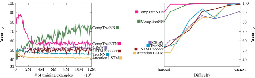
Figure 5, left panel, provides further insights into these results by tracking dev-set performance throughout training. It is evident here that the standard models never get traction on the prob-lem. The volatility of the CompTreeNN and CompTreeNTN is also again evident. Notably, the CompTreeNN is the only model that doesn’t peak in the first four training epochs, showing steady improvement throughout training.

We can also increase the number of training ex-amples so that the training data redundantly en-codes the information needed for fairness. As we do this, the learning problem becomes one of trivial memorization. Figure 5, right panel, tracks performance on this sequence of progres-sively more trivial problems. The CompTreeNN and CompTreeNTN both rapidly ascend to perfect performance. In contrast, the four standard mod-els continue to have largely undistinguished per-formance for all but the most trivial problems. Fi-nally, CBoW, while competitive with other neural

models initially, falls behind in a permanent way; its inability to account for word order prevents it from even memorizing the training data.

The results in Figure 5 are for models trained to predict the semantic relations for every subex-pression pair in the scope of a node in the tree in Figure 3 (as discussed in Section 5), but we also trained the models without intermediate pre-dictions to quantify their impact.

All models fail on our difficult generalization task when these intermediate values are withheld. Without intermediate values this task is unfair by our standards, so this to be expected. In the hard-est generalization setting the CBoW model is the only one of the four standard models to show sta-tistically significant improvement when interme-diate predictions are made. We hypothesize that the model is learning relations between open-class lexical items, which are more easily accessible in its sentence representations. As the general-ization task approaches a memorgeneral-ization task, the four standard models benefit more and more from intermediate predictions. In the easiest general-ization setting, the four standard models are un-able to achieve a perfect solution without inter-mediate predictions, while the CompTreeNN and CompTreeNTN models achieve perfection with or without the intermediate values. Geiger et al.

(2018) show that this is due to standard models being unable to learn the lexical relations between open class lexical items when not directly trained on them. Even with intermediate predictions, the standard models are only able to learn the base case of this recursive composition.

7 The Problem is Architecture

Attention LSTM TreeNN LSTM EncoderCBoW CompTreeNTN CompTreeNN

0 2M 4M 6M 8M 10M 12M ·104

33 40 50 60 70 80 90 100

# of training examples

Accurac

y

Attention LSTM TreeNN LSTM Encoder CBoW CompTreeNTN

CompTreeNN

hardest easiest

40 50 60 70 80 90 100

Difficulty

Accurac

y

Figure 5:Left: Model performance on our difficult but fair generalization task throughout training.Right: Mean accuracy of 5 runs as we move from true generalization tasks (‘hardest’) to problems in which the training set contains so much redundant encoding of the test set that the task is essentially one of memorization (‘easiest’). Only the task-specific CompTreeNN and CompTreeNTN are able to do well on true generalization tasks. The other neural models succeed only where memorization suffices, and the CBoW model never succeeds because it does not encode word order.

the trends by epoch and final results are virtually identical with 200-dimensional rather than 100-dimensions representations.

The reason these standard neural models fail to perform natural logic reasoning is their architec-ture. The CBoW, TreeNN, and LSTM Encoder models all separately bottleneck the premise and hypothesis sentences into two sentence vector em-beddings, so the only place interactions between the two sentences can occur is in the two hid-den layers before the softmax layer. However, the essence of natural logic reasoning is recursive composition up a tree structure where the premise and hypothesis are composed jointly, so this bot-tleneck proves extremely problematic. The At-tention LSTM model has an architecture that can align and combine lexical items from the premise and hypothesis, but it cannot perform this process recursively and also fails. The CompTreeNN and CompTreeNTN have this recursive tree structure encoded as hard alignments in their architecture, resulting in higher performance. Perhaps in future work, a general purpose model will be developed that can learn to perform this recursive composi-tion without a hard-coded aligned tree structure.

8 Conclusion and Future Work

It is vital that we stress-test our models of seman-tics using methods that go beyond standard nat-uralistic corpus evaluations. Recent experiments with artificial and adversarial example generation have yielded valuable insights here already, but it is vital that we ensure that these evaluations are fair in the sense that they provide our

mod-els with achievable, unambiguous learning targets. We must carefully and precisely navigate the bor-der between meaningful difficulty and impossibil-ity. To this end, we developed a formal notion of fairness for train/test splits.

This notion of fairness allowed us to rigorously pose the question of whether specific NLI models can learn to do robust natural logic reasoning. For our standard models, the answer is no. For our task-specific models, which align premise and hy-pothesis, the answer is more nuanced; they do not achieve perfect performance on our task, but they do much better than standard models. This helps us trace the problem to the information bottleneck formed by learning separate premise and hypoth-esis representations. This bottleneck prevents the meaningful interactions between the premise and hypothesis that are at the core of inferential rea-soning with language. Our task-specific models are cumbersome for real-world tasks, but they do suggest that truly robust models of semantics will require much more compositional interaction than is typical in today’s standard architectures.

Acknowledgments

References

Johan van Benthem. 2008. A brief history of natu-ral logic. InLogic, Navya-Nyaya and Applications: Homage to Bimal Matilal.

Samuel R. Bowman. 2013. Can recursive neural ten-sor networks learn logical reasoning? CoRR, abs/1312.6192.

Samuel R. Bowman, Gabor Angeli, Christopher Potts, and Christopher D. Manning. 2015a. A large anno-tated corpus for learning natural language inference. In Proceedings of the 2015 Conference on Empiri-cal Methods in Natural Language Processing, pages 632–642, Lisbon, Portugal. Association for Compu-tational Linguistics.

Samuel R. Bowman, Christopher Potts, and Christo-pher D. Manning. 2015b.Recursive neural networks can learn logical semantics. InProceedings of the 3rd Workshop on Continuous Vector Space Models and their Compositionality, pages 12–21. Associa-tion for ComputaAssocia-tional Linguistics.

Ishita Dasgupta, Demi Guo, Andreas Stuhlm¨uller, Samuel J. Gershman, and Noah D. Goodman. 2018.

Evaluating compositionality in sentence embed-dings.CoRR, abs/1802.04302.

Jeffrey L. Elman. 1990. Finding structure in time. Cognitive Science, 14(2):179–211.

Richard Evans, David Saxton, David Amos, Pushmeet Kohli, and Edward Grefenstette. 2018. Can neu-ral networks understand logical entailment? CoRR, abs/1802.08535.

Atticus Geiger, Ignacio Cases, Lauri Karttunen, and Christopher Potts. 2018. Stress-testing neural mod-els of natural language inference with multiply-quantified sentences. Ms., Stanford University. arXiv 1810.13033.

Max Glockner, Vered Shwartz, and Yoav Goldberg. 2018. Breaking nli systems with sentences that re-quire simple lexical inferences. InProceedings of the 56th Annual Meeting of the Association for Com-putational Linguistics (Volume 2: Short Papers), pages 650–655. Association for Computational Lin-guistics.

Ian J. Goodfellow, Jonathon Shlens, and Christian Szegedy. 2015. Explaining and harnessing adver-sarial examples. InICLR.

Suchin Gururangan, Swabha Swayamdipta, Omer Levy, Roy Schwartz, Samuel Bowman, and Noah A. Smith. 2018. Annotation artifacts in natural lan-guage inference data. InProceedings of the 2018 Conference of the North American Chapter of the Association for Computational Linguistics: Human Language Technologies, Volume 2 (Short Papers), pages 107–112. Association for Computational Lin-guistics.

Sepp Hochreiter and J¨urgen Schmidhuber. 1997. Long short-term memory. Neural Comput., 9(8):1735– 1780.

Thomas F. Icard and Lawrence S. Moss. 2013. Recent progress on monotonicity. Linguistic Issues in Lan-guage Technology, 9(7):1–31.

Robin Jia and Percy Liang. 2017. Adversarial exam-ples for evaluating reading comprehension systems. In Proceedings of the 2017 Conference on Empiri-cal Methods in Natural Language Processing, pages 2021–2031, Copenhagen, Denmark. Association for Computational Linguistics.

Diederik P. Kingma and Jimmy Ba. 2014. Adam: A method for stochastic optimization. CoRR, abs/1412.6980.

Brenden M. Lake and Marco Baroni. 2017. Still not systematic after all these years: On the composi-tional skills of sequence-to-sequence recurrent net-works.CoRR, abs/1711.00350.

Bill MacCartney and Christopher D. Manning. 2007.

Natural logic for textual inference. InProceedings of the ACL-PASCAL Workshop on Textual Entail-ment and Paraphrasing, RTE ’07, pages 193–200, Stroudsburg, PA, USA. Association for Computa-tional Linguistics.

Bill MacCartney and Christopher D. Manning. 2009.

An extended model of natural logic. InProceedings of the Eight International Conference on Compu-tational Semantics, pages 140–156. Association for Computational Linguistics.

W. McCune. 2005–2010. Prover9 and Mace4.http:

//www.cs.unm.edu/˜mccune/prover9/.

Aakanksha Naik, Abhilasha Ravichander, Norman Sadeh, Carolyn Rose, and Graham Neubig. 2018. Stress test evaluation for natural language inference. arXiv preprint arXiv:1806.00692.

Yixin Nie, Yicheng Wang, and Mohit Bansal. 2018. Analyzing compositionality-sensitivity of NLI mod-els. CoRR, abs/1811.07033.

Adam Poliak, Jason Naradowsky, Aparajita Haldar, Rachel Rudinger, and Benjamin Van Durme. 2018.

Hypothesis only baselines in natural language in-ference. In Proceedings of the Seventh Joint Con-ference on Lexical and Computational Semantics, pages 180–191. Association for Computational Lin-guistics.

Tim Rockt¨aschel, Edward Grefenstette, Karl Moritz Hermann, Tom´as Kocisk´y, and Phil Blunsom. 2015.

Reasoning about entailment with neural attention. CoRR, abs/1509.06664.

Richard Socher, Cliff Chiung-Yu Lin, Andrew Y. Ng, and Christopher D. Manning. 2011a. Parsing natu-ral scenes and natunatu-ral language with recursive neu-ral networks. In Proceedings of the 28th Interna-tional Conference on InternaInterna-tional Conference on Machine Learning, ICML’11, pages 129–136, USA. Omnipress.

Richard Socher, Jeffrey Pennington, Eric H. Huang, Andrew Y. Ng, and Christopher D. Manning. 2011b.

Semi-supervised recursive autoencoders for predict-ing sentiment distributions. InProceedings of the Conference on Empirical Methods in Natural Lan-guage Processing, EMNLP ’11, pages 151–161, Stroudsburg, PA, USA. Association for Computa-tional Linguistics.

Richard Socher, Alex Perelygin, Jean Wu, Jason Chuang, Christopher D. Manning, Andrew Ng, and Christopher Potts. 2013. Recursive deep models for semantic compositionality over a sentiment tree-bank. In Proceedings of the 2013 Conference on Empirical Methods in Natural Language Process-ing, pages 1631–1642, Seattle, Washington, USA. Association for Computational Linguistics.

Christian Szegedy, Wojciech Zaremba, Ilya Sutskever, Joan Bruna, Dumitru Erhan, Ian Goodfellow, and Rob Fergus. 2014. Intriguing properties of neural networks. InInternational Conference on Learning Representations.

Masatoshi Tsuchiya. 2018. Performance impact caused by hidden bias of training data for recogniz-ing textual entailment. CoRR, abs/1804.08117.

Sara Veldhoen and Willem Zuidema. 2018. Can neural networks learn logical reasoning? InProceedings of the Conference on Logic and Machine Learning in Natural Language (LaML 2017), pages 35–41. As-sociation for Computational Linguistics.