Orthonormal Explicit Topic Analysis for Cross-lingual Document Matching
John Philip McCrae University Bielefeld
Inspiration 1 Bielefeld, Germany
Philipp Cimiano University Bielefeld
Inspiration 1 Bielefeld, Germany
{jmccrae,cimiano,rklinger}@cit-ec.uni-bielefeld.de Roman Klinger University Bielefeld
Inspiration 1 Bielefeld, Germany
Abstract
Cross-lingual topic modelling has applications in machine translation, word sense disam-biguation and terminology alignment. Multi-lingual extensions of approaches based on la-tent (LSI), generative (LDA, PLSI) as well as explicit (ESA) topic modelling can induce an interlingual topic space allowing documents in different languages to be mapped into the same space and thus to be compared across languages. In this paper, we present a novel approach that combines latent and explicit topic modelling approaches in the sense that it builds on a set of explicitly defined top-ics, but then computes latent relations between these. Thus, the method combines the ben-efits of both explicit and latent topic mod-elling approaches. We show that on a cross-lingual mate retrieval task, our model signif-icantly outperforms LDA, LSI, and ESA, as well as a baseline that translates every word in a document into the target language.
1 Introduction
Cross-lingual document matching is the task of, given a query document in some source language, estimating the similarity to a document in some tar-get language. This task has important applications in machine translation (Palmer et al., 1998; Tam et al., 2007), word sense disambiguation (Li et al., 2010) and ontology alignment (Spiliopoulos et al., 2007). An approach that has become quite popular in re-cent years for cross-lingual document matching is Explicit Semantics Analysis (ESA, Gabrilovich and Markovitch (2007)) and its cross-lingual extension
CL-ESA (Sorg and Cimiano, 2008). ESA indexes documents by mapping them into a topic space de-fined by their similarity to predede-fined explicit top-ics – generally articles from an encyclopaedia – in such a way that there is a one-to-one correspondence between topics and encyclopedic entries. CL-ESA extends this to the multilingual case by exploiting a background document collection that is aligned across languages, such as Wikipedia. A feature of ESA and its extension CL-ESA is that, in contrast to latent (e.g. LSI, Deerwester et al. (1990)) or genera-tive topic models (such as LDA, Blei et al. (2003)), it requires no training and, nevertheless, has been demonstrated to outperform LSI and LDA on cross-lingual retrieval tasks (Cimiano et al., 2009).
A key choice in Explicit Semantic Analysis is the document space that will act as the topic space. The standard choice is to regard all articles from a back-ground document collection – Wikipedia articles are a typical choice – as the topic space. However, it is crucial to ensure that these topics cover the se-mantic space evenly and completely. In this pa-per, we present an alternative approach where we remap the semantic space defined by the topics in such a manner that it is orthonormal. In this way, each document is mapped to a topic that is distinct from all other topics. Such a mapping can be con-sidered as equivalent to a variant of Latent Seman-tic Indexing (LSI) with the main difference that our model exploits the matrix that maps topic vectors back into document space, which is normally dis-carded in LSI-based approaches. We dub our model
ONETA(OrthoNormal Explicit Topic Analysis) and empirically show that on a cross-lingual retrieval
task it outperforms ESA, LSI, and Latent Dirichlet Allocation (LDA) as well as a baseline consisting of translating each word into the target language, thus reducing the task to a standard monolingual match-ing task. In particular, we quantify the effect of dif-ferent approximation techniques for computing the orthonormal basis and investigate the effect of vari-ous methods for the normalization of frequency vec-tors.
The structure of the paper is as follows: we situate our work in the general context of related work on topic models for cross-lingual document matching in Section 2. We present our model in Section 3 and present our experimental results and discuss these results in Section 4.
2 Related Work
The idea of applying topic models that map docu-ments into an interlingual topic space seems a quite natural and principled approach to tackle several tasks including the cross-lingual document retrieval problem.
Topic modelling is the process of finding a rep-resentation of a documentdin a lower dimensional spaceRKwhere each dimension corresponds to one
topicthat abstracts from specific words and thus al-lows us to detect deeper semantic similarities be-tween documents beyond the computation of the pure overlap in terms of words.
Three main variants of document models have been mainly considered for cross-lingual document matching:
Latent methods such as Latent Semantic Indexing (LSI, Deerwester et al. (1990)) induce a de-composition of the term-document matrix in a way that reduces the dimensionality of the documents, while minimizing the error in re-constructing the training data. For example, in Latent Semantic Indexing, a term-document matrix is approximated by a partial singu-lar value decomposition, or in Non-Negative Matrix Factorization (NMF, Lee and Seung (1999)) by two smaller non-negative matrices. If we append comparable or equivalent doc-uments in multiple languages together before computing the decomposition as proposed by Dumais et al. (1997) then the topic model is
essentially cross-lingual allowing to compare documents in different languages once they have been mapped into the topic space.
Probabilistic or generative methods instead at-tempt to induce a (topic) model that has the highest likelihood of generating the documents actually observed during training. As with la-tent methods, these topics are thus interlin-gual and can generate words/terms in differ-ent languages. Prominent representatives of this type of method are Probabilistic Latent Se-mantic Indexing (PLSI, Hofmann (1999)) or Latent Dirichlet Allocation (LDA, Blei et al. (2003)), both of which can be straightforwardly extended to the cross-lingual case (Mimno et al., 2009).
Explicit topic models make the assumption that topics are explicitly given instead of being in-duced from training data. Typically, a back-ground document collection is assumed to be given whereby each document in this corpus corresponds to one topic. A mapping from doc-ument to topic space is calculated by comput-ing the similarity of the document to every doc-ument in the topic space. A prominent exam-ple for this kind of topic modelling approach is Explicit Semantic Analysis (ESA, Gabrilovich and Markovitch (2007)).
3 Orthonormal explicit topic analysis
Our approach follows Explicit Semantic Analysis in the sense that it assumes the availability of a back-ground document collection B = {b1, b2, ..., bN}
consisting of textual representations. The map-ping into the explicit topic space is defined by a language-specific function Φthat maps documents intoRN such that thejthvalue in the vector is given by someassociation measureφj(d)for each
back-ground documentbj. Typical choices for this
associ-ation measureφare the sum of the TF-IDF scores or an information retrieval relevance scoring function such as BM-25 (Sorg and Cimiano, 2010).
For the case of TF-IDF, the value of thej-th ele-ment of the topic vector is given by:
φj(d) =
−−−→
tf-idf(bj)T
−−−→
tf-idf(d)
Thus, the mapping function can be represented as the product of a TF-IDF vector of documentd multi-plied by anW×Nmatrix,X, each element of which contains the TF-IDF value of wordiin documentbj:
Φ(d) =
−−−→
tf-idf(b1)T
.. . −−−→
tf-idf(bN)T
−−−→
tf-idf(d) =XT·−−−→tf-idf(d)
For simplicity, we shall assume from this point on that all vectors are already converted to a TF-IDF or similar numeric vector form. In order to com-pute the similarity between two documents di and
dj, typically the cosine-function (or the normalized
dot product) between the vectorsΦ(di)andΦ(dj)is
computed as follows:
sim(di, dj) = cos(Φ(di),Φ(dj)) =
Φ(di)TΦ(dj)
||Φ(di)||||Φ(dj)||
If we represent the above using our above defined W ×N matrixXthen we get:
sim(di, dj) = cos(XTdi,XTdj) =
dTiXXTdj
||XTd
i||||XTdj||
The key challenge with ESA is choosing a good background document collectionB ={b1, ..., bN}.
A simple minimal criterion for a good background document collection is that each document in this
collection should be maximally similar to itself and less similar to any other document:
∀i6=j 1 = sim(bj, bj)>sim(bi, bj)≥0
While this criterion is trivially satisfied if we have no duplicate documents in our collection, our intu-ition is that we should choose a background collec-tion that maximizes theslack marginof this inequal-ity, i.e. |sim(bj, bj)−sim(bi, bj)|. We can see that
maximizing this margin for all i,j is the same as minimizing thesemantic overlapof the background documents, which is given as follows:
overlap(B) = X
i= 1, . . . , N j= 1, . . . , N
i6=j
sim(bi, bj)
We first note that we can, without loss of general-ity, normalize our background documents such that
||Xbj|| = 1 for all j, and in this case we can
re-define the semantic overlap as the following matrix expression1
overlap(X) =||XTXXTX−I||1
It is trivial to verify that this equation has a mini-mum whenXTXXTX =I. This is the case when the topics areorthonormal:
(XTbi)T(XTbj) = 0 ifi6=j
(XTbi)T(XTbi) = 1
Unfortunately, this is not typically the case as the documents have significant word overlap as well as semantic overlap. Our goal is thus to apply a suitable transformation toX with the goal of ensuring that the orthogonality property holds.
Assuming that this transformation of X is done by multiplication with some other matrixA, we can define the learning problem as finding that matrixA such that:
(AXTX)T(AXTX) =I
1||
A||p=Pi,j|aij|pis thep-norm. ||A||F =
If we have the case thatW ≥N and that the rank ofX is N, then XTX is invertible and thus A = (XTX)−1is the solution to this problem.2
We define the projection function of a document d, represented as a normalized term frequency vec-tor, as follows:
ΦONETA(d) = (XTX)−1XTd
For the cross-lingual case we assume that we have two sets of background documents of equal size, B1 = {b11, . . . , b1N}, B2 = {b21, . . . , b2N} in lan-guages l1 and l2, respectively and that these
doc-uments are aligned such that for every index i, b1i and b2i are documents on the same topic in each language. Using this we can construct a projec-tion funcprojec-tion for each language which maps into the same topic space. Thus, as in CL-ESA, we obtain the cross-lingual similarity between a document di
in languagel1 and a documentdj in languagel2 as
follows:
sim(di, dj) = cos(ΦlONETA1 (di),ΦlONETA2 (dj))
We note here that we assume thatΦcould be rep-resented as a symmetric inner product of two vec-tors. However, for many common choices of asso-ciation measures, including BM25, this is not the case. In this case the expression XTX can be re-placed with a kernel matrix specifying the associ-ation of each background document to each other background document.
3.1 Relationship to Latent Semantic Indexing
In this section we briefly clarify the relationship be-tween our method ONETA and Latent Semantic In-dexing. Latent Semantic Indexing defines a map-ping from a document represented as a term fre-quency vector to a vector in RK. This transforma-tion is defined by means of calculating the singu-lar value decomposition (SVD) of the matrix X as above, namely
2
In the case that the matrix is not invertible we can in-stead solve||XTXA−I||F, which has a minimum atA =
VΣ−1UT
whereXTX = UΣVT
is the singular value de-composition ofXTX.
As usual we do not in fact compute the inverse for our exper-iments, but instead the LU Decomposition and solve by Gaus-sian elimination at test time.
X=UΣVT
WhereΣis diagonal andU Vare the eigenvec-tors ofXXTandXTX., respectively. LetΣK
de-note the K ×K submatrix containing the largest eigenvalues, andUK,VKdenote the corresponding
eigenvectors. Thus LSI can be defined as:
ΦLSI(d) =Σ−K1UKd
With regards to orthonormalized topics, we see that using the SVD, we can simply derive the fol-lowing:
(XTX)−1XT=VΣ−1UT
When we setK =N and thus choose the maxi-mum number of topics, ONETA is equivalent to LSI modulo the fact that it multiplies the resulting topic vector by V, thus projecting back into document space, i.e. into explicit topics.
In practice, both methods differ significantly in that the approximations they make are quite differ-ent. Furthermore, in the case thatW N andX hasnnon-zeroes, the calculation of the SVD is of complexityO(nN +W N2)and requiresO(W N)
bytes of memory. In contrast, ONETA requires com-putation time ofO(Na)fora >2, which is the com-plexity of the matrix inversion algorithm3, and only
O(n+N2)bytes of memory.
3.2 Approximations
The computation of the inverse has a complexity that, using current practical algorithms, is approxi-mately cubic and as such the time spent calculating the inverse can grow very quickly. There are sev-eral methods for obtaining an approximate inverse. The most commonly used are based on the SVD or eigendecomposition of the matrix. AsXTXis sym-metric positive definite, it holds that:
XTX=UΣUT
WhereUare the eigenvectors ofXTXandΣis a diagonal matrix of the eigenvalues. WithUK,ΣK
3Algorithms witha= 2.3727are known but practical
as the firstK eigenvalues and eigenvectors, respec-tively, we have:
(XTX)−1 'UKΣ−K1UTK (1)
We call this the orthonormal eigenapproxima-tion or ON-Eigen. The complexity of calculating
(XTX)−1XT from this isO(N2K +N n), where nis the number of non-zeros inX.
Similarly, using the formula derived in the previ-ous section we can derive an approximation of the full model as follows:
(XTX)−1XT 'UKΣ−K1VTK (2)
We call this approximationExplicit LSI as it first maps into the latent topic space and then into the explicit topic space.
We can consider another approximation by notic-ing that X is typically very sparse and moreover some rows ofXhave significantly fewer non-zeroes than others (these rows are for terms with low fre-quency). Thus, if we take the firstN1columns
(doc-uments) in X, it is possible to rearrange the rows of X with the result that there is some W1 such
that rows with index greater thanW1 have only
ze-roes in the columns up toN1. In other words, we
take a subset of N1 documents and enumerate the
words in such a way that the terms occurring in the first N1 documents are enumerated1, . . . , W1. Let
N2 =N −N1,W2 =W −W1. The result of this
row permutation does not affect the value ofXTX
and we can write the matrixXas:
X=
A B
0 C
whereAis aW1×N1 matrix representing term
frequencies in the firstN1documents,Bis aW1×
N2 matrix containing term frequencies in the
re-maining documents for terms that are also found in the firstN1documents, andCis aW2×N2
contain-ing the frequency of all terms not found in the first N1documents.
Application of the well-known divide-and-conquer formula (Bernstein, 2005, p. 159) for matrix inversion yields the following easily verifi-able matrix identity, given that we can findC0 such thatC0C=I.
(ATA)−1AT −(ATA)−1ATBC0
0 C0
A B
0 C
=I
(3)
We denote the above equation using a matrix L as LTX = I. We note that L = (6 XTX)−1X, but for any document vectordthat is representable as a linear combination of the background doc-ument set (i.e., columns of X) we have that Ld = (XTX)−1XTd and in this sense L '
(XTX)−1XT.
We further relax the assumption so that we only need to find a C0 such that C0C ' I. For this, we first observe thatCis very sparse as it contains only terms not contained in the firstN1 documents
and we notice that very sparse matrices tend to be approximately orthogonal, hence suggesting that it should be very easy to find a left-inverse ofC. The following lemma formalizes this intuition:
Lemma: IfCis a W ×N matrix withM non-zeros, distributed randomly and uniformly across the matrix, and all the non-zeros are 1, thenDCTChas an expected value on each non-diagonal value of NM2 and a diagonal value of1ifDis the diagonal matrix whose values are given by||ci||−2, the square of the
norm of the corresponding column ofC.
Proof: We simply observe that ifD0 =DCTC, then the(i, j)th element ofD0is given by
dij =
cTi cj
||ci||2
Ifi 6= jthen the cTi cj is the number of non-zeroes
overlapping in theithandjthcolumn ofCand under a uniform distribution we expect this to beMN32. Sim-ilarly, we expect the column norm to be MN such that the overall expectation is NM2. The diagonal value is clearly equal to1.
As long as Cis very sparse, we can use the fol-lowing approximation, which can be calculated in
O(M) operations, whereM is the number of non-zeroes.
C0'
||c1||−2 0
. ..
0 ||cN2||
−2
C
T
Document Normalization
Frequency Normalization No Yes
TF 0.31 0.78
Relative 0.23 0.42
TFIDF 0.21 0.63
[image:6.612.72.292.59.166.2]SQRT 0.28 0.66
Table 1: Effect of Term Frequency and Document Nor-malization on Top-1 Precision
order O(N1a), being much more efficient than the eigenvalue methods. However, it is potentially more error-prone as it requires that a left-inverse ofC ex-ists. On real data this might be violated if we do not have linear independence of the rows ofC, for ex-ample ifW2 < N2or if we have even one document
which has only words that are also contained in the first N1 documents and hence there is a row in C
that consists of zeros only. This can be solved by removing documents from the collection until Cis row-wise linear independent.4
3.3 Normalization
A key factor in the effectiveness of topic-based methods is the appropriate normalization of the el-ements of the document matrix X. This is even more relevant for orthonormal topics as the matrix inversion procedure can be very sensitive to small changes in the matrix. In this context, we con-sider two forms of normalization, term and docu-ment normalization, which can also be considered as row/column normalizations ofX.
A straightforward approach to normalization is to normalize each column of Xto obtain a matrix as follows:
X0 =
x1
||x1||
. . . xN
||xN||
If we calculateX0TX0 = Ythen we get that the
(i, j)-th element ofYis:
yij =
xTi xj
||xi||||xj||
4
In the experiments in the next section we discarded 4.2% of documents atN1= 1000and 47% of documents atN1= 5000
● ●
● ●
● ●
● ● ● ●
● ●
● ● ● ● ●
● ●
●
100 200 300 400 500
0.0
0.2
0.4
0.6
0.8
Approximation rate
Precision
● ● ●
● ●
● ●
● ●
● ●
● ● ● ●
● ● ● ● ● ●
●
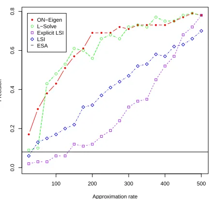
[image:6.612.318.535.75.281.2]− ON−Eigen L−Solve Explicit LSI LSI ESA
Figure 1: Effect on Top-1 Precision by various approxi-mation method
Thus, the diagonal ofY consists of ones only and due to the Cauchy-Schwarz inequality we have that
|yij| ≤ 1, with the result that the matrix Y is
al-ready close toI. Formally, we can use this to state a bound on||X0TX0−I||F, but in practice it means
that the orthonormalizing matrix has more small or zero values.
A further option for normalization is to consider some form of term frequency normalization. For term frequency normalization, we use TF (tfwn), Relative(tfwn
Fw ),TFIDF (tfwnlog(
N
dfw)), andSQRT (√tfwn
Fw). Here,tfwn is the term frequency of wordw in document n, Fw is the total frequency of word
w in the corpus, and dfw is the number of
docu-ments containing the words w. The first three of these normalizations have been chosen as they are widely used in the literature. The SQRT normaliza-tion has been shown to be effective for explicit topic methods in previous experiments not reported here.
4 Experiments and Results
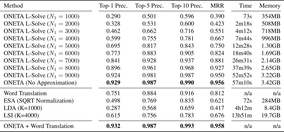
Method Top-1 Prec. Top-5 Prec. Top-10 Prec. MRR Time Memory
ONETA L-Solve (N1= 1000) 0.290 0.501 0.596 0.390 73s 354MB ONETA L-Solve (N1= 2000) 0.328 0.531 0.600 0.423 2m18s 508MB ONETA L-Solve (N1= 3000) 0.462 0.662 0.716 0.551 4m12s 718MB ONETA L-Solve (N1= 4000) 0.599 0.755 0.781 0.667 7m44s 996MB ONETA L-Solve (N1= 5000) 0.695 0.817 0.843 0.750 12m28s 1.30GB ONETA L-Solve (N1= 6000) 0.773 0.883 0.905 0.824 18m40s 1.69GB ONETA L-Solve (N1= 7000) 0.841 0.928 0.937 0.881 26m31s 2.14GB ONETA L-Solve (N1= 8000) 0.896 0.961 0.968 0.927 37m39s 2.65GB ONETA L-Solve (N1= 9000) 0.924 0.981 0.987 0.950 52m52s 3.22GB ONETA (No Approximation) 0.929 0.987 0.990 0.956 57m10s 3.42GB
Word Translation 0.751 0.884 0.916 0.812 n/a n/a ESA (SQRT Normalization) 0.498 0.769 0.835 0.621 72s 284MB LDA (K=1000) 0.287 0.568 0.659 0.417 4h12m 8.4GB LSI (K=4000) 0.615 0.756 0.783 0.676 13h51m 19.7GB
[image:7.612.72.530.55.269.2]ONETA + Word Translation 0.932 0.987 0.993 0.958 n/a n/a
Table 2: Result on large-scale mate-finding studies for English to Spanish matching
the similarity of the query document to all indexed documents, we compute the valueranki indicating
at which position the mate of theith document oc-curs. We use two metrics: Top-k Precision, defined as the percentage of documents for which the mate is retrieved among the firstkelements, andMinimum Reciprocal Rank, defined as
MRR = X
i∈test
1 ranki
For our experiments, we first extracted a subset of documents (every 20th) from Wikipedia, filtering this set down to only those that have aligned pages in both English and Spanish with a minimum length of 100 words. This gives us 10,369 aligned doc-uments in total, which form the background docu-ment collectionB. We split this data into a training and test set of 9,332 and 1,037 documents, respec-tively. We then removed all words whose total fre-quencies were below 50. This resulted in corpus of 6.7 millions words in English and 4.2 million words in Spanish.
Normalization Methods: In order to investigate the impact of different normalization methods, we ran small-scale experiments using the first 500 doc-uments from our dataset to train ONETA and then evaluate the resulting models on the mate-finding task on 100 unseen documents. The results are pre-sented in Table 1, which shows the Top-1 Precision
for the different normalization methods. We see that the effect of applying document normalization in all cases improves the quality of the overall result. Surprisingly, we do not see the same result for fre-quency normalization yielding the best result for the case where we do no normalization at all5. In the re-maining experiments we thus employ document nor-malization and no term frequency nornor-malization.
Approximation Methods: In order to evaluate the different approximation methods, we experimen-tally compare 4 different approximation methods: standard LSI, ON-Eigen (Equation 1), Explicit LSI (Equation 2), L-Solve (Equation 3) on the same small-scale corpus. For convenience we plot an ap-proximation ratewhich is eitherKorN1depending
on method; atK = 500 andN1 = 500, these
ap-proximations become exact. This is shown in Figure 1. We also observe the effects of approximation and see that the performance increases steadily as we increase the computational factor. We see that the orthonormal eigenvector (Equation 1) method and the L-solve (Equation 3) method are clearly simi-lar in approximation quality. We see that the explicit LSI method (Equation 2) and the LSI method both perform significantly worse for most of the
approxi-5A likely explanation for this is that low frequency terms are
mation amounts. Explicit LSI is worse than the other approximations as it first maps the test documents into aK-dimensional LSI topic space, before map-ping back into theN-dimensional explicit space. As expected this performs worse than standard LSI for all but high values ofK as there is significant error in both mappings. We also see that the (CL-)ESA baseline, which is very low due to the small number of documents, is improved upon by even the least ap-proximation of orthonormalization. In the remain-ing of this section, we report results usremain-ing the L-Solve method as it has a very good performance and is computationally less expensive than ON-Eigen.
Evaluation and Comparison: We compare
ONETA using the L-Solve method withN1 values
from 1000 to 9000 topics with (CL-)ESA (using SQRT normalization), LDA (using 1000 topics) and LSI (using 4000 topics). We choose the largest topic count for LSI and LDA we could to provide the best possible comparison. For LSI, the choice of K was determined on the basis of operating system memory limits, while for LDA we experimented with higher values forK without any performance improvement, likely due to overfitting. We also stress that for L-Solve ONETA,N1 is not the topic
count but an approximation rate of the mapping. In all settings we useN topics as with standard ESA, and so should not be considered directly comparable to theKvalues of these methods.
We also compare to a baseline system that re-lies on word-by-word translation, where we use the most likely single translation of a word as given by a phrase table generated by the Moses system (Koehn et al., 2007) on the EuroParl corpus (Koehn, 2005). Top 1, Top 5 and Top 10 Precision as well as Mean Reciprocal Rank are reported in Table 2.
Interestingly, even for a small number of docu-ments (e.g., N1 = 6000) our results improve both
the word-translation baseline as well as all other topic models, ESA, LDA and LSI in particular. We note that at this level the method is still efficiently computable and calculating the inverse in practice takes less time than training the Moses system. The significance for results (N1 ≥ 7000) have been
tested by means of a bootstrap resampling signifi-cance test, finding out that our results significantly improve on the translation base line at a 99% level.
Further, we consider a straightforward combina-tion of our method with the translacombina-tion system con-sisting of appending the topic vectors and the trans-lation frequency vectors, weighted by the relative average norms of the vectors. We see that in this case the translations continue to improve the perfor-mance of the system (albeit not significantly), sug-gesting a clear potential for this system to help in im-proving machine translation results. While we have presented results for English and Spanish here, simi-lar results were obtained for the German and French case but are not presented here due to space limita-tions.
In Table 2 we also include the user time and peak resident memory of each of these processes, mea-sured on an 8 Core Intel Xeon 2.50 GHz server. We do not include the results for Word Translation as many hours were spent learning a phrase table, which includes translations for many phrases not in the test set. We see that the ONETA method signif-icantly outperforms LSI and LDA in terms of speed and memory consumption. This is in line with the theoretical calculations presented earlier where we argued that inverting theN×N dense matrixXTX whenW N is computationally lighter than find-ing an eigendecomposition of the W ×W sparse matrix XXT. In addition, as we do not multiply
(XTX)−1 and XT, we do not need to allocate a large W ×K matrix in memory as with LSI and LDA.
The implementations of ESA, ONETA, LSI and LDA used as well as the data for the experiments are available at http://github.com/jmccrae/oneta.
5 Conclusion
while the induction of the model takes less time than training the machine translation system from a parallel corpus. We have also presented an effec-tive approximation method, i.e. L-Solve, which sig-nificantly reduces the computational cost associated with computing the topic models.
Acknowledgements
This work was funded by the Monnet Project and the Portdial Project under the EC Sev-enth Framework Programme, Grants No. 248458 and 296170. Roman Klinger has been funded by the “Its OWL” project (“Intelli-gent Technical Systems Ostwestfalen-Lippe”, http://www.its-owl.de/), a leading-edge cluster of the German Ministry of Education and Research.
References
Dennis S Bernstein. 2005. Matrix mathematics, 2nd Edi-tion. Princeton University Press Princeton.
David M Blei, Andrew Y Ng, and Michael I Jordan. 2003. Latent Dirichlet Allocation. Journal of Ma-chine Learning Research, 3:993–1022.
Philipp Cimiano, Antje Schultz, Sergej Sizov, Philipp Sorg, and Steffen Staab. 2009. Explicit versus la-tent concept models for cross-language information re-trieval. InIJCAI, volume 9, pages 1513–1518. Don Coppersmith and Shmuel Winograd. 1990. Matrix
multiplication via arithmetic progressions. Journal of symbolic computation, 9(3):251–280.
Scott C. Deerwester, Susan T Dumais, Thomas K. Lan-dauer, George W. Furnas, and Richard A. Harshman. 1990. Indexing by latent semantic analysis. JASIS, 41(6):391–407.
Chris Ding, Tao Li, and Wei Peng. 2006. NMF and PLSI: equivalence and a hybrid algorithm. In Pro-ceedings of the 29th annual international ACM SIGIR, pages 641–642. ACM.
Susan T Dumais, Todd A Letsche, Michael L Littman, and Thomas K Landauer. 1997. Automatic cross-language retrieval using latent semantic indexing. In AAAI spring symposium on cross-language text and speech retrieval, volume 15, page 21.
Evgeniy Gabrilovich and Shaul Markovitch. 2007. Com-puting semantic relatedness using Wikipedia-based ex-plicit semantic analysis. InProceedings of the 20th In-ternational Joint Conference on Artificial Intelligence, volume 6, page 12.
Thomas Hofmann. 1999. Probabilistic latent semantic indexing. InProceedings of the 22nd annual interna-tional ACM SIGIR conference, pages 50–57. ACM. Philipp Koehn, Hieu Hoang, Alexandra Birch, Chris
Callison-Burch, Marcello Federico, Nicola Bertoldi, Brooke Cowan, Wade Shen, Christine Moran, Richard Zens, et al. 2007. Moses: Open source toolkit for sta-tistical machine translation. InProceedings of the 45th Annual Meeting of the ACL, pages 177–180. Associa-tion for ComputaAssocia-tional Linguistics.
Philipp Koehn. 2005. Europarl: A parallel corpus for sta-tistical machine translation. InMT summit, volume 5. Daniel D Lee and H Sebastian Seung. 1999. Learning
the parts of objects by non-negative matrix factoriza-tion. Nature, 401(6755):788–791.
Linlin Li, Benjamin Roth, and Caroline Sporleder. 2010. Topic models for word sense disambiguation and token-based idiom detection. In Proceedings of the 48th Annual Meeting of the Association for Computa-tional Linguistics, pages 1138–1147. Association for Computational Linguistics.
David Mimno, Hanna M Wallach, Jason Naradowsky, David A Smith, and Andrew McCallum. 2009. Polylingual topic models. InProceedings of the 2009 Conference on Empirical Methods in Natural Lan-guage Processing, pages 880–889. Association for Computational Linguistics.
Martha Palmer, Owen Rambow, and Alexis Nasr. 1998. Rapid prototyping of domain-specific machine trans-lation systems. InMachine Translation and the Infor-mation Soup, pages 95–102. Springer.
Philipp Sorg and Philipp Cimiano. 2008. Cross-lingual information retrieval with explicit semantic analysis. InProceedings of the Cross-language Evaluation Fo-rum 2008.
Philipp Sorg and Philipp Cimiano. 2010. An experi-mental comparison of explicit semantic analysis im-plementations for cross-language retrieval. InNatural Language Processing and Information Systems, pages 36–48. Springer.
Vassilis Spiliopoulos, George A Vouros, and Vangelis Karkaletsis. 2007. Mapping ontologies elements us-ing features in a latent space. In IEEE/WIC/ACM International Conference on Web Intelligence, pages 457–460. IEEE.