Abstract— A Genetic Algorithm based multi-objective methodology was implemented for a self-organizing wireless sensor network. Design parameters such as network density, connectivity and energy consumption are taken into account for developing the fitness function. The genetic algorithm optimizes the operational modes of the sensor nodes along with clustering schemes and transmission signal strengths. The algorithm has been implemented in MATLAB using its Genetic Algorithm toolbox along with custom codes. The optimal designs so achieved by the algorithm conform to all the design parameters.
Index Terms – Genetic Algorithms, Network Configuration , Sensor Placement, Wireless Sensor Networks.
I. INTRODUCTION
A
dvancements in technologies such as Sensing, Electronics and Computing have attracted tremendous research interest in the field of Wireless Sensor Networks (WSNs), apart from their enormous potential for both commercial and military applications. A WSN generally consists of a large number of low-cost, low-power, multifunctional, energy constrained sensor nodes with limited computational and communication capabilities [1]. In WSNs sensors may be deployed either randomly or deterministically depending upon the application [2]. Deployment in a battlefield or hazardous areas is generally random, whereas a deterministic deployment is preferred in amicable environments. In general a deterministic placement requires fewer sensor nodes than the random deployment to perform the same task.Network lifetime is one of the important parameters to optimize as energy resources in a WSN are limited due to operation on battery. Replacing or recharging of battery in the network may be infeasible. Though the overall function of the
Manuscript received November 28, 2008.
*Amol P Bhondekar, is with the Central Scientific Instruments Organisation, Sector 30,Chandigarh-160030,INDIA (Phone:+91-172-2657811 ext.489;Fax:+91-172-2657082; e-mail: [email protected]
Renu Vig is with the University Institute of Engineering and Technology, Panjab University, Chandigarh 160025, INDIA ([email protected] ).
Madan Lal Singla, is with the Central Scientific Instruments Organisation, Sector 30,Chandigarh-160030,INDIA (e-mail: [email protected] )
C Ghanshyam is with the Central Scientific Instruments Organisation, Sector 30,Chandigarh-160030,INDIA (e-mail: [email protected] )
Pawan Kapur, is with the Central Scientific Instruments Organisation, Sector 30, Chandigarh 160030,INDIA (e-mail: [email protected] )
network may not be hampered due to failure one or few nodes of the network as neighboring nodes may take over, but for optimum performance the network density must be high enough. Network connectivity which depends upon the communication protocol is another WSN design issue. Generally cluster based architecture is followed by the most common protocol. In cluster-based architecture, the nodes are grouped in clusters which communicate with a sink node; the sink node gathers information from the nodes in its cluster and transmits the information to the base station. Network connectivity issues include the number of sensor nodes in a cluster depending upon the load handling capability of the sink nodes, as well as the ability of sensor nodes to reach these sinks. Apart from the design issues discussed above some parameters depend upon the application for which the network is to be deployed. Although, several algorithms [2]-[16] have been proposed for design optimization of WSNs but many of them fail to address the application specific issues. Consideration of the application specific issues makes the design optimization much more complex.
The above mentioned issues call for simultaneous optimization of more than one nonlinear design criteria, and the underlying challenge is to find as many near-optimal and non-dominant solutions as possible in unimpeachable computational constraints. Several interesting approaches like Neural Networks, Artificial Intelligence, Swarm Optimization, and Ant Colony Optimization have been implemented to tackle such problems. Genetic Algorithm (GA) is one of the most powerful heuristics for solving optimization problems that is based on natural selection, the process that drives biological evolution. The GA repeatedly modifies a population of individual solutions. At each step, the genetic algorithm selects individuals at random from the current population to be parents and uses them to produce the children for the next generation. Over successive generations, the population "evolves" towards an optimal solution. GAs can be applied to solve a variety of optimization problems that are not well suited for standard optimization algorithms, including problems in which the objective function is discontinuous, non-differentiable, stochastic, or highly nonlinear.
Several researchers have successfully implemented GAs in a sensor network design [17]-[23], this led to the development of several other GA-based application-specific approaches in WSN design, mostly by the construction of a single fitness function. However, these approaches either cover limited network characteristics or fail to incorporate several application specific requirements into the performance measure of the heuristic.In this work we have tried to integrate
Genetic Algorithm Based Node Placement
Methodology For Wireless Sensor Networks
network characteristics and application specific requirements in the performance measure of the GA. The algorithm primarily finds the operational modes of the nodes in order to meet the application specific requirements along with minimization of energy consumption by the network. More specifically, network design is investigated in terms of active sensors placement, clustering and communication range of sensors, while performance estimation includes, together with connectivity and energy-related characteristics, some application-specific properties like uniformity and spatial density of sensing points. Thus, the implementation of the proposed methodology results in an optimal design scheme, which specifies the operation mode for each sensor.
II. METHODOLOGY
This work assumes a hypothetical application which involves deployment of three types of sensors on a two dimensional field for monitoring of hypothetical parameters say X, Y and Z. It is assumed that spatial variability
ρ
x,ρ
y,ρ
z of parameters X ,Y and Z respectively, are such thatρ
x<<y
ρ
<<ρ
z. It means that the variation of X in the 2D field is much less than Y and the variation Y is much less than Z. i.e. the density of sensor nodes monitoring Z has to be more than Y and density of sensor nodes monitoring Y has to be more than X in order to optimally monitor the field. The methodology adopted herein not only takes into account the general network characteristics, but also the above described application specific characteristics.A. Problem Outline 1) Network Model
Consider a square field of L x L Euclidian units subdivided into grids separated by a predefined Euclidian distance. The sensing nodes are placed at the intersections of these grids so that the entire area of interest is covered (See Fig. 1).
Fig 1.A grid based wireless sensor network layout.
The sensing nodes are identical and assumed to have features like; power control, sensing mode selection (X, Y or Z) and transmission power control. The nodes are capable of selecting one of the three operating modes i.e. X sense, Y sense and Z sense provided they are active. The nodes operating in X sensing mode has the highest transmission range whereas
nodes in Y and Z sensing modes have medium and low transmission ranges respectively. Although several cluster based sophisticated methodologies have been proposed [25-27], we have adopted a simple cluster based architecture, wherein the nodes operating in X sense mode act as cluster-in-charge and are able to communicate with the base station (sink) via multihop communication and the clusters are formed based on the vicinity of sensors to the cluster-in-charge. The cluster-in-charge performs tasks such as data collection and aggregation at periodic intervals including some computations. It is very clear that the nodes in X sense mode will consume more power than the other two modes.
2) Problem Statement
Here we explore a multi-objective algorithm to design WSN topologies. The algorithm optimizes application specific parameters, connectivity parameters and energy parameters by using a single fitness function. This fitness function gives the quality measure of each WSN topology and further optimizes it to best topology. WSN design parameters can be broadly classified into three categories [23]. The first category colligates parameters regarding sensor deployment specifically, uniformity and coverage of sensing and measuring points respectively. The second category colligates the connectivity parameters such as number of cluster-in-charge and the guarantee that no node remains unconnected. The third category colligates the energy related parameters such as the operational energy consumption depending on the types of active sensors. The design optimization is achieved by minimizing constraints such as, operational energy, number of unconnected sensors and number of overlapping cluster- in-charge ranges. Whereas the parameters such as, field coverage and number of sensors per cluster-in-charge are to be maximized. A weighted sum approach has been used to aggregate all these optimization constraints and an objective function is formed as given by the equation (1) below, this objective function is the basis for forming the “fitness function” for the GA and gives an numerical figure for quality measure of each possible solution of the optimization problem.
=
∑
= 5
1
min
i i i
P
k
f
(1)Where, ki is the corresponding weight Pi is the optimization parameter
TABLE I
Correspondences between objectives and optimization parameters
Objective Optimization Parameters Symbols
P1 Field Coverage FC
P2 Overlaps per cluster-in-charge error OpCiE
P3 Sensor out of range error SORE
P4 Sensors per cluster-in-charge SpCi
B. Optimization Parameters
1) Application-specific parameter: Theeffectiveness of a distributed WSN highly depends upon the sensor deployment scheme. It is highly desirable to deploy the sensing nodes such that maximum field coverage and high quality communication is achieved. Here, a field coverage parameter is defined as under:
total
inactive OR
z y x
n
n
n
n
n
n
FC
=
(
+
+
)
−
(
+
)
(2)Where, x
n
number of X Sensors (cluster-in-charge) yn
number of Y Sensorsz
n
number of Z Sensors ORn
number of Out of Range Sensors inactiven
number of Inactive Sensors totaln
total number of sensing points2) Connectivityparameters: Perpetual network connectivity is a crucial issue in WSNs. Following parameters are taken into account for reliable network connectivity:
(a) A Sensors-per-Cluster-in-charge (SpCi) parameter which ascertains that each cluster-in-charge does not earmark sensors more than its traffic handling, data management and the sensor physical communication capabilities:
ch OR z y
n
n
n
n
SpCi
=
+
−
(3)(b) A Sensors-Out-of-Range Error (
SORE
) parameter to ascertain that each sensor gets included in a cluster. This of course depends on the communication range of the sensor nodes. It is assumed that Y mode sensors cover a circular area with radius equal to 2 2 length units, while Z mode sensorscover a circular area with radius equal to 2 length units.
SORE
is given by :inactive total
OR
n
n
n
SORE
−
=
(4)(c) A Overlaps-per-cluster-in-charge error (
OpCiE
) parameter which ensures that the cluster-in-charges are so distributed or chosen such that there is a minimum overlapping of cluster-in-charge ranges, i.e to ensure that a sensor remains loyal to one cluster-in-charge only.OpCiE
is given by:x
n
overlaps
of
number
OpCiE
=
_
_
(5)
3) Energy-related parameter: Energy consumption is a crucial issue affecting the overall performance of a WSN in terms of reliability and life time. An optimization parameter
defined as Network Energy (NE) is taken into consideration here, which is a numerical measure of energy consumption depending on a network design. It basically depends on the operational modes of the sensing nodes, sensors operating in X mode (cluster-in-charge) will obviously consume the highest energy as they require high communication power and perform data aggregation and scheduling tasks, the nodes operating in Y mode consume less power than X mode as their communication range is less than X mode and the Z mode nodes will consume the lowest power as they have lowest communication range. Here, it is assumed that a node in X mode consumes 4 times power than in Z mode and node in Y mode consumes 2 times more power than in Z mode. Hence the NE consumption parameter is given by:
total z y x
n
n
n
n
NE
=
4
.
+
2
.
+
(6)C. WSN representation
As described in previous section a square field of L xL length units is considered which is subdivided into grids of unit lengths. The nodes are assumed to be placed on intersections of these grids. An individual in GA population is represented by a bit-string and is used to encode sensor nodes in a row by row fashion as shown in Fig. 2.
Fig 2.Bit string representation of network layout.
The length of this bit string is 2.L2 as two bits are required to encode four types of sensing nodes i.e. X, Y, Z and inactive nodes. In this bit string the sequence of two bits decides the type of node 00 being inactive, 01 being X mode, 10 being Y mode and 11 represents Z mode. Thus if the value of L is 10 then the length of the bit string would be 200. In Fig. 2, L is 5 and hence the length of bit string is 50.
D. Fitness function, Genetic Operators and Selection Mechanism
design parameters. The fitness function is minimized by the GA system in the process of evolutionary optimization. Having described the design parameters we formalize our fitness function as:
NE SpCi SORE
OpCiE FC
f =−α1 +α2 +α3 −α4 +α5 (7)
It may be noted that the coefficients
α
1 andα
4have negative signs, this is because the GA toolbox of MATLAB optimizes the problem by minimizing the fitness value and in order to maximize the parameters corresponding to these particular coefficients they have to be multiplied by a negative sign. In this fitness function the significance of each design parameter is defined by setting appropriate weighting coefficientsα
i: i = 1, 2. . . 5. The values of these coefficients were determined based on design requirements and experimentation. Initially all the coefficients were set to unity and the significance of each of the parameter was determined after some rudimentary GA runs. The optimized values of the weights were hence obtained and importance of each design parameter was set.TABLE II
Optimized Values of Weighing Coefficients
Parameter Coefficient Optimized Value
Field Coverage α
1 4
Overlaps-per-cluster-in-charge error
α
2 0.5
Sensors-Out-of-Range error α
3 10
Sensors-per-cluster-in-charge
α
4 1
Network Energy α
5 1
As can be seen in Table 2, the final weights were such that network connectivity parameters (weights α1, α4) were treated as constraints, in the sense that all sensors should be in range with a cluster in-charge and no cluster in-charge should be connected to more than the predefined number of sensors nodes.
GA optimization procedure highly depends on the crossover and mutation methodologies. The crossover methodologies available in the GA toolbox of MATLAB are scattered, single point, two point, intermediate and heuristic. However, the two point crossover methodology was used as it gave us optimum performance in terms of time and speed. This two point methodology selects two random integers m and n
between 1 and number of variables. The algorithm selects genes numbered less than or equal to m from the first parent, selects genes numbered from m+1 to n from the second parent, and selects genes numbered greater than n from the first parent. The algorithm then concatenates these genes to form a single gene.
The mutation methodologies available in GA toolbox of MATLAB are Gaussian and Uniform. Gaussian methodology adds a random number to each vector entry of an individual. This random number is taken from a Gaussian distribution centered on zero. The variance of this distribution can be
controlled with two parameters. The Scale parameter determines the variance at the first generation. The Shrink parameter controls how variance shrinks as generations go by. If the Shrink parameter is 0, the variance is constant. If the Shrink parameter is 1, the variance shrinks to 0 linearly as the last generation is reached, however the Gaussian mutation methodology was used with a scale and shrink factor of 1. Four elite individuals (individuals with the best fitness values) of each generation were chosen in order to ensure that the current best individuals always survived to the next generation.
III. EXPERIMENTAL RESULTS
GAs involves exploration and tuning of a number of problem specific parameters for optimizing its performance, namely the population size, crossover and mutation methodologies. Firstly, a number of experiments were conducted to determine appropriate population size, size ranging from 100 to 1000 individuals. However, the best performance, by means of maximizing the corresponding fitness function, was achieved with a population size of 300 individuals. Then, several explorations were performed with different crossover methodologies as discussed in previous section; the best performing crossover methodology i.e the two point methodology with a crossover fraction of 0.8 was selected. Similarly, a Gaussian mutation methodology with scale and shrink factor of 1 was found to give the best performance. Due to the stochasticity of GAs during optimization, the quality of the randomly generated initial population plays an important role in the final performance. Thus, several runs were tested with different random initial populations. Average results over the several runs as well as the best solutions achieved by each set of parameters were used to draw conclusions. The developed algorithm was tested in following way. First, the performance of the algorithm in designing initial optimal WSN topologies and sensor operation modes was examined.
Thus, the algorithm was applied in a field of 10 x 10 sensing nodes assuming full battery capacity. The algorithm was started, having available all sensor nodes of the grid at full battery capacities. The three GA runs that gave the best results after 3000 generations were recorded and their results are discussed here (abbreviated as ‘‘GA1’’, ‘‘GA2’’ and ‘‘GA3’’, starting from the fittest design). The evolution progress of the best GA run is shown in Fig. 3, where both the fitness progress of the best individual found by the algorithm as well as the average fitness of the entire population at each generation are plotted. The optimization in the entire GA population can be seen from the general minimization of the average population fitness, despite the numerous fluctuations caused by the search process through the genetic operators of crossover and mutation.
Circles with a cross mark represent an out of range sensor node and an empty space represent an inactive sensor node.
Fig 3.Evolution progress of the best individual (best fitness value) and the entire population (average fitness value) of the
GA during the two best runs of the algorithm.
Fig 4.Graphical representation of one of the networks optimized by the algorithm
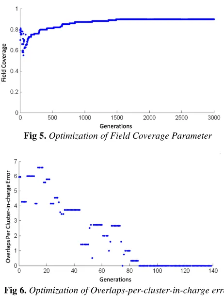
The optimization performed by the GA evolution process can also be seen by the progress of the values of some of the parameters of the WSN designs found during the evolution. Fig.5 is plot of evolution of field coverage parameter (FC)
during the optimization of the designs till the 3000th generation. It is quite evident form Fig. 6 that the algorithm tries to increase the field coverage in the successive generations and converges at an optimum value which is well above the 0.8 mark (80%).
The evolution of Overlaps-per-cluster-in-charge error (
OpCiE
)parameter is shown in Fig.6. It is quite evident that the algorithm tries to minimize the error and is successful in making it zero during the first 100 generations of the evolution. The evolution of Sensors-Out-of-Range Error (SORE
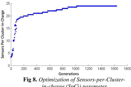
) parameter is shown in Fig. 7, wherein during the initial generations the algorithm randomly selects the individuals and the SORE parameter varies randomly, but as the evolution proceeds this parameter is optimized and goesbelow the 0.1 mark(10%). The evolution of Sensors-per- Cluster-in-charge (SpCi) parameter is shown in Fig 8. The algorithm tries to maximize this parameter during the evolution and it was observed that almost in every run of the
Fig 5.Optimization of Field Coverage Parameter
Fig 6.Optimization of Overlaps-per-cluster-in-charge error
(
OpCiE
)parameterFig 7.Optimization of Sensors-Out-of-Range Error (
SORE
) parameter [image:5.595.50.281.129.262.2] [image:5.595.306.537.139.444.2] [image:5.595.54.284.331.489.2]random designs suffered with communication limitation issues, the algorithm at the beginning of the evolution was always
Fig 8.Optimization of Sensors-per-Cluster-in-charge (SpCi) parameter
trying to find designs that at least satisfied the communication and the application-specific constraints. Table 3 shows the details on all sensor network characteristics for the three GA- generated designs. Figures 10, 11 and 12 show the layout design of GA1, GA2 and GA3 respectively.
Fig 9.Optimization of Network Energy Parameter
TABLE III
Optimized Parameter Values for the three GA-Generated Network Layouts
Design Parameter GA1 GA2 GA3
FC 0.8 0.7 0.9
OpCiE 0 0 0
SORE 0 0 0
SpCi 21.5 20.25 22.75
NE 2.24 2.21 2.46
Active Sensors 90 85 95
X Mode Sensors 4 4 4
Y Mode sensors 58 60 75
Z Mode Sensors 28 21 16
Inactive Sensors 10 15 5
Out of Range Sensors 0 0 0
X Mode Sensors/Active Sensors 0.044 0.047 0.042
Y Mode Sensors/Active Sensors 0.640 0.705 0.789
Z Mode Sensors/Active Sensors 0.311 0.247 0.168
Fitness -22.46 -20.84 -23.89
[image:6.595.330.518.99.706.2]Fig 10.Network Layout of GA1
Fig 11.Network Layout of GA2
[image:6.595.44.263.129.275.2] [image:6.595.48.285.377.753.2] [image:6.595.337.516.388.690.2]IV. CONCLUSIONS
In this paper we have demonstrated the use of genetic algorithm based node placement methodology for a wireless sensor network. A fixed wireless network of sensors of different operating modes was considered on a grid deployment and the GA system decided which sensors should be active, which ones should operate as cluster-in-charge and whether each of the remaining active normal nodes should have medium or low transmission range. The network layout design was optimized by taking into consideration application specific parameter, connectivity parameters and energy related parameters. From the evolution of network characteristics during the optimization process, we can conclude that it is preferable to operate a relatively high number of sensors and achieve lower energy consumption for communication purposes than having less active sensors with consequently larger energy consumption for communication purposes. In addition, GA-generated designs compared favorably to random designs of sensors. Uniformity of sensing points of optimal designs was satisfactory, while connectivity constraints were met and operational and communication energy consumption was minimized. We also showed that dynamic application of the algorithm in WSN layout design can lead to the extension of the network’s life span, while keeping the application-specific properties of the network close to optimal values. The algorithm showed sophisticated characteristics in the decision of sensors’ activity/inactivity schedule as well as the rotation of operating modes (X, Y & Z modes). But there still exists lot of scope for future work to deal with the development of heuristic methodologies for optimal routing of dynamically selected cluster-in-charge sensors, through some multi-hop communication protocols. Also, methodologies could be developed for dynamic integration of battery capacity.
REFERENCES
[1] I.F. Akyildiz, W. Su, Y. Sankarasubramaniam, E. Cayirci, “Wireless sensor networks: a survey”, Computer Networks 38(2002), pp. 393– 422.
[2] M. Ishizuka, M. Aida, “Performance study of node placement in sensor networks,” in: Proc. of 24th International Conference on Distributed Computing Systems Workshops, 2004, pp. 598–603.
[3] S. Slijepcevic, M. Potkonjak, “Power efficient organization of wireless sensor networks”, in: Proc. IEEE Int. Conf. on Communications, Helsinki, Finland, 2001, pp. 472–476.
[4] B. Krishnamachari, F. Ordo´nez, “Analysis of energy-efficient, fair routing in wireless sensor networks through non-linear optimization”, in: Proc. IEEE Vehicular Technology Conference– Fall, Orlando, FL, 2003, pp. 2844–2848.
[5] C. Zhou, B. Krishnamachari, “Localized topology generation mechanisms for wireless sensor networks”, in: IEEE GLOBECOM’ 03, San Francisco, CA, December 2003.
[6] S.Y. Chen, Y.F. Li, “Automatic sensor placement for model based robot vision”, IEEE Trans. Syst. Man Cyber. 34 (Feb) (2004) pp. 393–408. [7] A. Trigoni, Y. Yao, A. Demers, J. Gehrke, R. Rajaraman, “Wave
Scheduling: energy-efficient data dissemination for sensor networks”, in: Proc. Int. Workshop on Data Management for Sensor Networks (DMSN), in conjunction with VLDB, 2004.
[8] S. Ghiasi, A. Srivastava, X. Yang, M. Sarrafzadeh, “Optimal energy aware clustering in sensor networks”, Sensors 2 (2002), pp. 258–269. [9] V. Rodoplu, T.H. Meng, Minimum energy mobile wireless networks,
IEEE J. Select. Areas Commun. 17 (8) (1999), pp. 1333–1344.
[10] J.-H. Chang, L. Tassiulas, “Energy conserving routing in wireless ad-hoc networks”, in: Proc. IEEE INFOCOM’00, Tel Aviv, Israel, 2000, pp. 22–31.
[11] D.J. Chmielewski, T. Palmer, V. Manousiouthakis, “On the theory of optimal sensor placement”, AlChE J. 48 (5) (2002), pp. 1001–1012. [12] A. Arbel, “Sensor placement in optimal filtering and smoothing
problems”, IEEE Trans. Automat. Control 27 (February) (1982), pp. 94– 98.
[13] H. Zhang, “Two-dimensional optimal sensor placement”, IEEE Trans. Syst. Man Cyber. 25 (May) (1995), pp. 781–792.
[14] K. Chakrabarty, S.S. Iyengar, H. Qi, E. Cho, “Grid coverage for surveillance and target location in distributed sensor networks”, IEEE Trans. Comput. 51 (December) (2002), pp. 1448–1453.
[15] S.S. Dhillon, K. Chakrabarty, ‘‘Sensor placement for effective coverage and surveillance in distributed sensor networks’’, in: Proc. of IEEE Wireless Communications and Networking Conference, vol. 3, March 2003, pp. 1609–1614.
[16] V. Mhatre, C. Rosenberg, D. Kofman, R. Mazumdar, N. Shroff, “A minimum cost heterogeneous sensor network with a lifetime constraint”, IEEE Trans. Mobile Comput. 4 (1) (2005), pp. 4–15.
[17] S. Sen, S. Narasimhan, K. Deb, “Sensor network design of linear processes using genetic algorithms”, Comput. Chem. Eng. 22 (3) (1998), pp. 385–390.
[18] S.A. Aldosari, J.M.F. Moura, “Fusion in sensor networks with communication constraints”, in: Information Processing in Sensor Networks (IPSN’04), Berkeley, CA, April 2004.
[19] D. Turgut, S.K. Das, R. Elmasri, B. Turgut, “Optimizing clustering algorithm in mobile ad hoc networks using genetic algorithmic approach”, in: IEEE GLOBECOM’02, Taipei,Taiwan, November 2002. [20] G. Heyen, M.-N. Dumont, B. Kalitventzeff, “Computer-aided design of
redundant sensor networks”, in: Escape 12, The Aague, The Netherlands, May 2002.
[21] S. Jin, M. Zhou, A.S. Wu, “Sensor network optimization using a genetic algorithm”, in: 7th World Multiconference on Systemics, Cybernetics and Informatics, Orlando, FL, 2003.
[22] D.B. Jourdan, O.L. de Weck, “Layout optimization for a wireless sensor network using a multi-objective genetic algorithm”, in: IEEE Semiannual Vehicular Technology Conference, Milan, Italy, May 2004. [23] Konstantinos P. Ferentinos, Theodore A. Tsiligiridis, “Adaptive design
optimization of wireless sensor networks using genetic algorithms”, Computer Networks 51 (2007),pp. 1031–1051
[24] K. Sohrabi, J. Gao, V. Ailawadhi, G.J. Pottie, “Protocols for self-organization of a wireless sensor network”, IEEE Personal Commun. Mag. 7 (5) (2000), pp. 16–27.
[25] O. Younis, S. Fahmy, “Distributed clustering in ad-hoc sensor networks: a hybrid, energy-efficient approach”, in: INFOCOM 2004, Hong Kong, March, 2004.
[26] M. Younis, M. Youssef, K. Arisha, “Energy-aware routing in cluster-based sensor networks”, in: 10th IEEE/ACM International Symposium on Modeling, Analysis and Simulation of Computer and Telecommunication Systems (MASCOTS 2002), Fort Worth, TX, October 2002.