Assessment of Cold Wind Creation and Flow for Improving Urban Amenity

(1)

https://www.scirp.org/journal/jep ISSN Online: 2152-2219

ISSN Print: 2152-2197

DOI: 10.4236/jep.2019.1011082 Nov. 1, 2019 1391 Journal of Environmental Protection

Assessment of Cold-Wind Creation and Flow for

Improving Urban Amenity

Daewuk Kim1*, Kyungsu Son1, Sanghun Baek1, Eungho Jung2

1_{R & D Center, New Layer Co., Ltd., Daegu, Korea}

2_{Department of Environmental Planning, Keimyung University, Daegu, Korea}

Abstract

This study is intended to recognize the importance of cold-wind, which is one of the solutions to improve urban amenity, and verify the model that can analyze creation and flow of cold-wind. For this reason, KLAM_21 Model, which was developed by the German’s Meteorological Service, was selected and used for assessment of cold-wind creation and flow. As a result, the followings have been drawn through comparison with measured data and simulated data in the study area; for a mountain area, the simulation result of velocity and direction of wind has been indicated as similar as those in meas-ured data. For a stream area in the city, only wind direction from simulation has been consistent with measured data whereas wind velocity showed a large difference between measurement and simulation. Finally, for the downtown area, wind velocity has shown a lot of differences between simulation result and measured data. Wind direction has also shown a large difference until midnight. But after midnight, model data have become similar as measured data. According to the verification of this study, the model used in this study for using urban-amenity improvement through assessment of creation and flow of cold wind is suitable to analyze the direction of cold wind that is gen-erated in the periphery of the city and the overall flow within the existing ur-ban area. But the results of wind velocity have shown the uppermost limit of the modeling in the simulation. That is, it could not reflect the site characte-ristics sufficiently. Therefore, if parameters considering the specific regional characteristics are sufficiently reflected, the result of simulations for reliability can be substantially improved.

Keywords

Urban Amenity, Cold Wind, Fresh Air, KLAM_21, Model Evaluation

How to cite this paper: Kim, D., Son, K., Baek, S. and Jung, E. (2019) Assessment of Cold-Wind Creation and Flow for Im-proving Urban Amenity. Journal of Envi-ronmental Protection, 10, 1391-1406.

https://doi.org/10.4236/jep.2019.1011082

Received: October 1, 2019 Accepted: October 29, 2019 Published: November 1, 2019

http://creativecommons.org/licenses/by/4.0/

(2)

DOI: 10.4236/jep.2019.1011082 1392 Journal of Environmental Protection

1. Introduction

Currently, computer applications or computer simulations are widely utilized to minimize damage related to urban development by predicting and evaluating the environmental effects due to urban development in advance. In particular, cold air or a wind path has been applied to improve urban amenity in Korea and oth-er nations in reality. Thus, various models [1] [2] [3] [4] [5] utilizing computa-tion fluid dynamics (CFD) have been developed and used practically and wind tunnel experiments have been conducted in parallel to verify the effect [6] [7] [8]

[9] [10]. However, few studies have been conducted on models that analyzed

creation and flow of cold air or fresh air around urban areas and evaluations on models.

In this study, a single evaluation model was selected based on spatial hierarchy and functional similarity with regard to evaluation models, which have been employed in study literatures in Korea and other nations up until today and computer simulations were conducted utilizing the evaluation model with re-gard to specific target regions. The simulation results were compared with measured data and a level of reliability was investigated. The aim of this study is to conduct pre-evaluation on urban development through reliable model utiliza-tion in the future.

2. Theoretical Discussion

2.1. Urban Amenity and Cold Air

1) Definition of urban amenity

Urban amenity means that residents in urban space can live and act safely and comfortably in general. This term was first used in the UK in terms of urban planning in the mid-19th century to early 20th century to indicate a core mean-ing “a residential area or city that is livable and comfortable and pleasant to live”. The term “amenity” in residential areas is interpreted that it is ensured when not only arrangement of living environmental facilities (roads, water supply and sewage systems, parks etc.) but also other factors that provide daily living with comfort (high dimensional and cultural requirements such as elimi-nation of noise, daily sunlight, greenery, privacy, or scenery, or cleanliness) [11].

2) Evaluation index of urban amenity

(3)

[image:3.595.210.536.89.234.2]

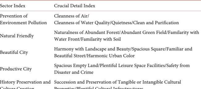
Table 1. Planning Indices for Urban Amenity in the wide level.

Sector Index Crucial Detail Index Prevention of

Environment Pollution

Cleanness of Air/

Cleanness of Water Quality/Quietness/Clean and Purification

Natural Friendly Naturalness of Abundant Forest/Abundant Green Field/Familarity with _{Water Front/Familarity with Soil}

Beautiful City Harmony with Landscape and Beauty/Spacious Square/Familiar and _{Beautiful Street/Harmonic Urban Color}

Productive City Spacious Empty Land/Plentiful Leisure Space Facilities/Safety from Disaster and Crime

History Preservation and

Culture Creation Succession and Preservation of Tangible or Intangible Cultural Properties/Plentiful Cultural Infrastructures

As such, “cleanness of air” is included in the indices that improve urban amenity. To maintain and improve clean air, cold air or fresh wind created in urban green fields and flown into cities is needed.

3) Cold air for improvement of urban amenity

One of the most known environmental problems in cities is an urban heat island. Due to urban heat island, comfort of life for residents in cities is degraded significantly. One of the solutions to the urban heat island can be cold wind mentioned in the above.

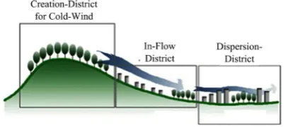
Cold wind is characterized that it is created from mountain areas around cities and flows into urban areas due to differences in height of terrains (refer to

“Figure 1”). This is a natural convection phenomenon occurred due to

differ-ences in specific heat between natural and artificial land covers. That is, hot air during the daytime in cities meet with highly dense cold air descended from the surrounding area after sunset, which moves hot air into the upper layer thereby incurring a natural circulation. Through this process, urban air can maintain cleanness and furthermore, urban amenity can be improved.

2.2. KLAM_21 Model for Analysis of Cold Wind Creation and Flow

1) Overview of KLAM_21

KLAM_21 (Kaltluftabflussmodell_21) is a model for cold wind creation and flow simulation test developed by the German Meteorological Agency, which is designed to analyzed and predict creation and flow of cold wind based on ter-rains and land usage. In addition, KLAM_21 was developed to provide basic data for pre-assessment or consultation of microclimate changes due to urban devel-opment or regional develdevel-opment [13].

(4)

[image:4.595.273.477.72.162.2]

Figure 1. Key map related to creation and flow of cold wind.

above information, a city size where simulations can be done is 37.5 × 37.5 km2_,

which can be highly useful model to see changes in microclimate due to urban development or regional development in a broad area. In addition to simulations of flow and creation of cold wind and expansion of pollution source, KLAM_21 can analyze a level of changes in wind flow due to barriers of block type. It has also nesting function, which is convenient to enlarge a cold wind flow in specific regions [14].

2) Operation method and process of KLAM_21

In order to perform simulation tests of cold wind creation and flow using KLAM_21, making a study area into a certain distance of grids shall be done first. Based on the grids, basic data must be inputted to enable efficient simula-tion tests as mensimula-tioned earlier. Next, topography data per grid as well as land cover data per grid are inputted simultaneously for data input. In the land cover classification, KLAM_21 divides land cover into nine classification standards basically. Each of land cover has its own attribute values such as the building coverage, length of roughness, wall index, height of trees, and relative radiant quantity. Whether cold wind is created or flows is determined based on the above attribute values.

Once the above grid process and data input process are complete, a script is created finally to perform simulation tests well. Here, types of simulation test results, storage interval of analysis and result are set up. Through the above processes, simulation test results of cold wind creation and flow can be derived. Based on this, cold air height and flow range in the study area as well as analysis results on cold air flow rate and direction can be obtained (refer to “Figure 2”).

3. Study Method

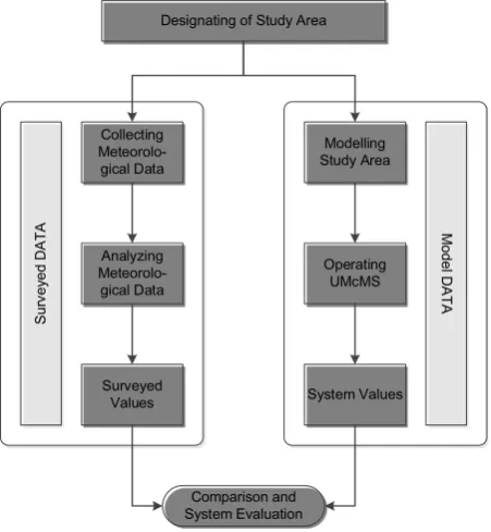
3.1. Flow of the Study

(5)

[image:5.595.259.487.68.307.2]

Figure 2. Operations and procedures of KLAM_21.

Figure 3. Flow chart of the Study.

3.2. Selection of Case Study Areas for Evaluation

In order to evaluate the analysis model of cold wind creation and flow accurate-ly, the study area was divided into one district in the mountain around the city where cold wind was created, two districts near the stream where cold wind flew to the city, and two districts in the existing downtown expected to have the cold wind effect. The detailed contents of the selected study area are as follows:

1) Location and overview of the measured locations in the study area Gridifying the Area

Inputting Data for each Grid

Draw-up of Script for Composing Simulation

Simulation

Analysis & Results of Creation and Flow of Cold-Air

for each Time

Analysis & Results of Directions and Wind-Speed of

Cold-Air for each Time

Topography Data Land-Cover Data

Time Saving Interval _{Parameter Value}Designating

Designating of Study Area

Collecting Meteorolo-gical Data

Modelling Study Area

Analyzing Meteorolo-gical Data

Operating UMcMS

Sur

vey

ed D

AT

A Mo

de

l DA

TA

Surveyed

Values System Values

[image:5.595.262.488.341.586.2]

(6)

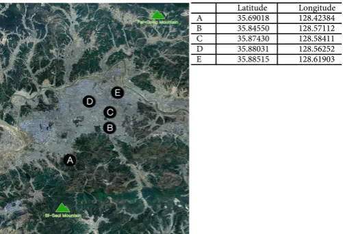
The study area was Daegu Metropolitan City according to the administrative district system and measured points were five locations: mountain area around the city (A point), around the stream in the city (B and C points), and existing downtown (D and E points). The study area was surrounded by Mt. Palgong to the north and Mt. Biseul to the south and gradual hills and fields in the east and west directions, which were relatively open space and places that were suitable to create cold and fresh wind due to the topographical conditions (refer to “Figure 4”).

2) General status of the study area a) Meteorological status of the study area

The study area is included in Daegu Metropolitan City according to the ad-ministrative district system as mentioned in the above. The meteorological status in Daegu Metropolitan City in the measured period (Aug. 10-Sep. 10 of 2016) showed that its average temperature was 27.9˚C and the maximum and mini-mum temperatures were 36.3˚C and 20.1˚C. The average cloudiness was 7.0 and total precipitation was 327.1 mm. The average wind velocity was 2.1 m/s and the maximum wind direction was normally east-southeasterly wind [15].

b) Land cover status by location in the study area

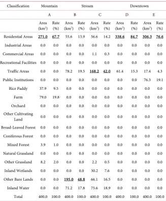
In order to investigate the land cover status by location in the study area, a range was set within a radius of 200 m in each point and the results were found by points according to the land cover classification standards in the Ministry of Environment, which are shown in “Table 2”.

[image:6.595.249.500.535.706.2]

A point, which was a mountain area near the city has the following land cover status. A low density residential area was the largest as 67.7% followed by field and paddies. B point, which was near the stream in the city, other bare lands ac-counted for 48.8%. C point showed that traffic area acac-counted for 42.0%, which was the largest, followed by inland water, which accounted for 18.9%. Finally, D and E points, which were existing downtowns, had densely populated residential areas, which accounted for 84.7% and 76.6% and showed typical land cover sta-tus of residential area.

Figure 4. Measuring points and its surrounding map within the study area.

(7)

[image:7.595.210.538.99.494.2]

Table 2. Status of land cover in the study area by standard classfication of the Ministry of

Environment in Korea.

Classification Mountain Stream Downtown

A B C D E

Area

(km2₎ Rate _(%) _(kmArea 2₎ Rate _(%) _(kmArea 2₎ Rate _(%) _(kmArea 2₎ Rate _(%) _(kmArea 2₎ Rate _(%) Residential Areas 271.0 67.7 55.6 13.9 56.6 14.2 338.6 84.7 306.3 76.6

Industrial Areas 0.0 0.0 0.0 0.0 0.0 0.0 0.0 0.0 0.0 0.0

Commercial Areas 0.0 0.0 0.0 0.0 1.1 0.3 0.0 0.0 0.0 0.0

Recreational Facilities 0.0 0.0 0.0 0.0 0.0 0.0 0.0 0.0 0.0 0.0 Traffic Areas 0.0 0.0 78.2 19.5 168.2 42.0 61.4 15.3 17.4 4.3 Public Institutions 0.0 0.0 0.0 0.0 0.0 0.0 0.0 0.0 76.3 19.1

Rice Paddy 37.9 9.5 0.0 0.0 0.0 0.0 0.0 0.0 0.0 0.0

Farm 79.0 19.8 0.0 0.0 0.0 0.0 0.0 0.0 0.0 0.0

Orchard 0.0 0.0 0.0 0.0 0.0 0.0 0.0 0.0 0.0 0.0

Other Cultivating

Land 0.0 0.0 0.0 0.0 0.0 0.0 0.0 0.0 0.0 0.0

Broad-Leaved Forest 0.0 0.0 0.0 0.0 0.0 0.0 0.0 0.0 0.0 0.0

Coniferous Forest 0.0 0.0 0.0 0.0 0.0 0.0 0.0 0.0 0.0 0.0

Mixed Forest 3.9 1.0 0.0 0.0 0.0 0.0 0.0 0.0 0.0 0.0

Natural Grassland 0.0 0.0 0.0 0.0 0.0 0.0 0.0 0.0 0.0 0.0

Other Grassland 8.2 2.0 0.0 0.0 2.2 0.5 0.0 0.0 0.0 0.0

Inland Wetlands 0.0 0.0 0.0 0.0 30.2 7.6 0.0 0.0 0.0 0.0

Other Bare Lands 0.0 0.0 195.0 48.8 66.1 16.5 0.0 0.0 0.0 0.0

Inland Water 0.0 0.0 71.2 17.8 75.6 18.9 0.0 0.0 0.0 0.0

Total 400.0 100.0 400.0 100.0 400.0 100.0 400.0 100.0 400.0 100.0

4. Evaluation of the Model

4.1. Analysis on Measured Data of the Study Area

1) Collection of measured data

In order to collect measured data of study area, Automatic Weather Station (AWS) devices were installed at all areas except for E area and meteorological data for one month from August 10 to September 10 in 2016 were collected. The detailed installation conditions are listed in “Table 3”, which are applied to all areas in the same manner. For E area, collected data at the AWS devices installed by the Korea Meteorological Administration (KMA) were extracted only for the same period and utilized in the analysis.

2) Analysis of measured data

(8)

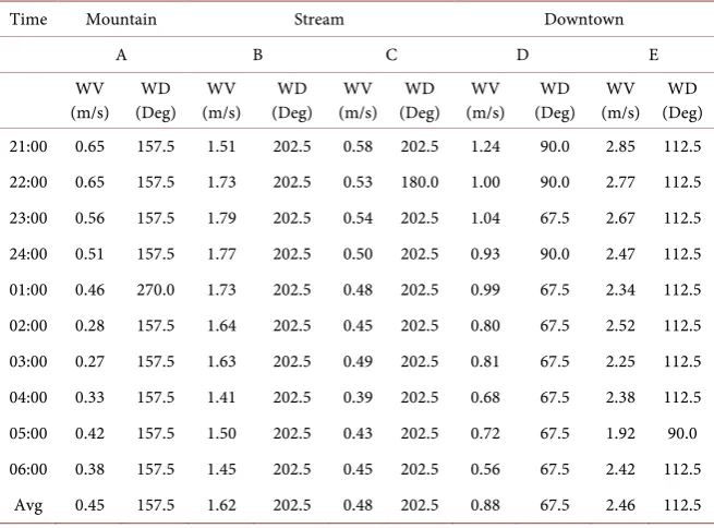
data of wind direction and velocity after 21:00 to 06:00 in the next day, in which cold wind was created and flown in terms of urban amenity, were found as shown in “Table 4”.

4.2. Analysis on Model Data of the Study Area

1) Simulation conditions for model data analysis a) Modelling conditions for simulation

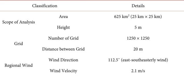
[image:8.595.208.539.374.440.2]

In order to analyze model data and collect result data, this study set the mountain point in the study area up to 25 km-long and 25 km-wide range and a height of model data were set to 5 m, which was the same installation height with the measuring equipment. The initial condition was set to store required data by dividing the area into 1250 in the horizontal direction and 1250 in the vertical direction by having a gap between grids to 20 m for modeling. In addi-tion, the input for regional wind that can consider accurate wind direction and velocity of fresh wind was set to wind direction of 112.5˚ (east-southeasterly wind) and wind velocity of 2.1 m/s based on the meteorological status in Daegu Metropolitan City. The simulation tests were conducted based on the above data (refer to “Table 5”).

Table 3. Installation of automatic weather station and collecting data.

Index Detail Information

Device Height 5 m above from Surface

Survey Period August 10, 2016-September 10, 2016

Collecting Data Wind Direction/Wind Velocity/Temperature

Table 4. Results of average wind direction and wind velocity during survey period.

Time Mountain Stream Downtown

A B C D E

WV

(m/s) (Deg) WD (m/s) WV (Deg) WD (m/s) WV (Deg) WD (m/s) WV (Deg) WD (m/s) WV (Deg) WD

21:00 0.65 157.5 1.51 202.5 0.58 202.5 1.24 90.0 2.85 112.5

22:00 0.65 157.5 1.73 202.5 0.53 180.0 1.00 90.0 2.77 112.5

23:00 0.56 157.5 1.79 202.5 0.54 202.5 1.04 67.5 2.67 112.5

24:00 0.51 157.5 1.77 202.5 0.50 202.5 0.93 90.0 2.47 112.5

01:00 0.46 270.0 1.73 202.5 0.48 202.5 0.99 67.5 2.34 112.5

02:00 0.28 157.5 1.64 202.5 0.45 202.5 0.80 67.5 2.52 112.5

03:00 0.27 157.5 1.63 202.5 0.49 202.5 0.81 67.5 2.25 112.5

04:00 0.33 157.5 1.41 202.5 0.39 202.5 0.68 67.5 2.38 112.5

05:00 0.42 157.5 1.50 202.5 0.43 202.5 0.72 67.5 1.92 90.0

06:00 0.38 157.5 1.45 202.5 0.45 202.5 0.56 67.5 2.42 112.5

Avg 0.45 157.5 1.62 202.5 0.48 202.5 0.88 67.5 2.46 112.5

[image:8.595.210.538.470.712.2]

(9)

[image:9.595.210.534.89.222.2]

Table 5. Modelling conditions for simulation of the study area.

Classification Details

Scope of Analysis Area 625 km

2_{(25 km × 25 km)}

Height 5 m

Grid Number of Grid 1250 × 1250

Distance between Grid 20 m

Regional Wind Wind Direction 112.5˚ (east-southeasterly wind)

Wind Velocity 2.1 m/s

b) Land cover classification and related parameters for simulation

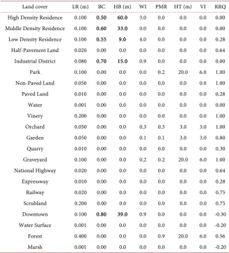
The land cover classification for simulation was based on the land cover classification in the Ministry of Environment and then reclassified according to the land cover classification standards required by the model as listed in

“Table 6”. The basic values in the model were used as the parameters

corres-ponding to each of land cover without change. Note that for high density resi-dence, mid-density resiresi-dence, low density resident, downtown, and industrial district, parameter values that corresponded to a building-to-land ratio and building height were modified and used on the basis of the current status data of buildings in Daegu Metropolitan City.

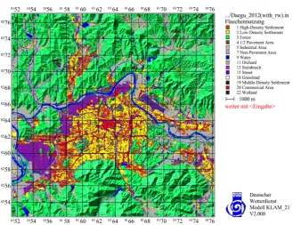
The result of land cover classification of the study area according to the above modeling conditions and land cover classification is shown in “Figure 5”.

2) Analysis of model data a) Result of the simulation

The results of the simulation tests by main hours derived through the above modeling are shown in “Table 7”. The table indicated overall that Mt. Palgong in the north and Mt. Biseul in the south formed fresh wind earnestly from 21H after the sunset at the surrounding mountain areas and the flow of the fresh wind had been stabilized after 24H gradually. The result of wind velocity showed that the base of the valley had faster wind velocity than other surround-ing areas.

b) Analysis of model data

“Table 8” shows the analysis result of model data by main hours, which

(10)

[image:10.595.209.537.88.449.2]

Table 6. Classification of land cover and relevant parameters for simulation.

Land cover LR (m) BC HB (m) WI PMR HT (m) VI RRQ

High Density Residence 0.100 0.50 60.0 3.0 0.0 0.0 0.0 0.00

Middle Density Residence 0.100 0.60 33.0 0.0 0.0 0.0 0.0 0.00

Low Density Residence 0.100 0.55 9.0 4.0 0.0 0.0 0.0 0.28

Half-Pavement Land 0.020 0.00 0.0 0.0 0.0 0.0 0.0 0.64

Industrial District 0.080 0.70 15.0 0.9 0.0 0.0 0.0 0.00

Park 0.100 0.00 0.0 0.0 0.2 20.0 6.0 1.00

Non-Paved Land 0.050 0.00 0.0 0.0 0.0 0.0 0.0 1.00

Paved Land 0.010 0.00 0.0 0.0 0.0 0.0 0.0 0.28

Water 0.001 0.00 0.0 0.0 0.0 0.0 0.0 0.00

Vinery 0.200 0.00 0.0 0.0 0.0 0.0 0.0 1.00

Orchard 0.050 0.00 0.0 0.3 0.3 3.0 3.0 1.00

Garden 0.050 0.00 0.0 0.1 0.1 3.0 3.0 0.80

Quarry 0.010 0.00 0.0 0.0 0.0 0.0 0.0 0.30

Graveyard 0.100 0.00 0.0 0.2 0.2 20.0 6.0 1.00

National Highway 0.020 0.00 0.0 0.0 0.0 0.0 0.0 0.64

Expressway 0.010 0.00 0.0 0.0 0.0 0.0 0.0 0.28

Railway 0.020 0.00 0.0 0.0 0.0 0.0 0.0 0.75

Scrubland 0.200 0.00 0.0 0.0 0.0 0.0 0.0 0.75

Downtown 0.100 0.80 39.0 0.9 0.0 0.0 0.0 -0.30

Water Surface 0.001 0.00 0.0 0.0 0.0 0.0 0.0 -0.20

Forest 0.400 0.00 0.0 0.0 0.9 20.0 6.0 0.56

Marsh 0.001 0.00 0.0 0.0 0.0 0.0 0.0 -0.20

LR: Length of Roughness, BC: Building Coverage, HB: Height of Building, WI: Wall Index, PMR: Plant Materials Rate, HT: Height of Trees, VI: Vertical Index, RRQ: Relative Radiant Quantity.

Table 7. Wind velocity & direction in the study area through simulation.

Time Results Time Results Legend

21H 03H

[image:10.595.197.538.499.735.2]

(11)

[image:11.595.210.540.89.377.2]

Table 8. Average wind directions & velocity through the simulation.

Time Mountain Stream Downtown

A B C D E

WV

(m/s) (Deg) WD (m/s) WV (Deg) WD (m/s) WV (Deg) WD (m/s) WV (Deg) WD (m/s) WV (Deg) WD

21:00 0.48 181.2 1.74 188.9 0.95 197.1 0.39 150.8 0.33 90.0

22:00 0.48 181.2 1.70 186.4 1.96 199.4 0.43 152.2 0.36 102.9

23:00 0.48 181.2 1.49 183.5 1.75 199.4 0.03 90.0 0.46 113.2

24:00 0.48 181.2 1.39 182.5 1.38 198.6 0.11 5.2 0.16 119.7

01:00 0.48 181.2 1.30 182.2 0.96 198.2 0.07 98.1 0.09 122.0

02:00 0.48 181.2 1.20 181.9 0.69 197.7 0.06 99.5 0.06 121.0

03:00 0.48 181.2 1.08 181.6 0.50 197.4 0.06 99.5 0.04 116.6

04:00 0.48 181.2 0.95 181.2 0.38 197.0 0.05 90.0 0.04 116.6

05:00 0.48 181.2 0.82 180.7 0.28 196.5 0.05 90.0 0.03 108.4

06:00 0.47 181.2 0.69 180.0 0.22 195.9 0.05 90.0 0.03 108.4

Avg 0.48 181.2 1.24 182.9 0.91 197.7 0.13 90.0 0.16 114.3

WV: Wind Velocity, WD: Wind Direction.

Figure 5. Land cover classification for simulation of the study area.

4.3. Evaluation on the Analysis Model

[image:11.595.209.539.406.659.2]

(12)

simulation tests were compared thereby deriving the result of evaluation on the cold wind creation and flow model, which is the ultimate object of this study.

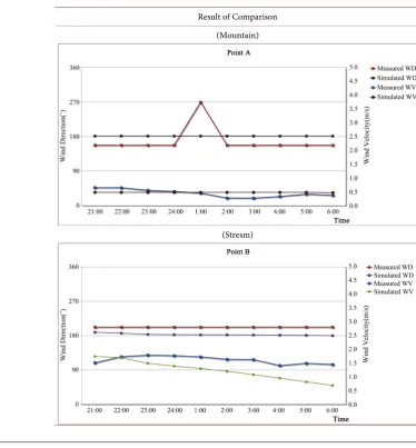
The overall results of wind velocity and direction showed that wind directions had highly similar results between measured and modeled data whereas wind velocities showed somewhat different results except for A point, which was a mountain area near the city.

[image:12.595.160.535.339.743.2]

The regional data results divided by mountain area around the city, stream area in the city, and existing downtown showed that a mountain area had similar results of wind direction and velocity between them and a stream area in the city had a slight difference in wind velocity but similar wind direction between two data. Finally, points of existing downtown showed that a wind velocity was much different from each other but wind direction indicated similar results ex-cept for some hour slots such as 24:00 and 1:00. These results are considered as good results considering the interference among various elements in the down-town (refer to “Table 9”).

Table 9. Comparison of wind velocity and directions for each time of surveyed data and

model data in study area.

Result of Comparison (Mountain)

(13)

Continued

(Stream)

(Downtown)

The above results were compared quantitatively, which are shown in Table 10. More specifically, the results are described as below:

(14)

area in the city, measured value of wind velocity was 1.62 m/s and that of model value was 1.24 m/s, resulting in a difference of 0.38 m/s whereas wind directions revealed similar results between measured value (south-southeasterly wind (202.5˚)) and model value (southerly wind (182.9˚)). For C point, a measured value of wind velocity was 0.48 m/s and model value was 0.91 m/s, indicating that a model value was 0.43 m/s higher than measured value whereas wind di-rection revealed nearly the same results between measured value (202.5˚) and model value (197.7˚).

[image:14.595.214.538.368.702.2]

For D point, which is existing downtown, a difference in wind velocity be-tween measured (0.88 m/s) and model (0.13 m/s) values was 0.75 m/s while wind direction showed a difference after sunset until the midnight but after 1:00 am the next day both of measured value (east northeasterly wind (67.5˚)) and model value (easterly wind (90.0˚)) had similar wind directions despite some difference to some extent. For E point, measured value (2.46 m/s) and model value (0.16 m/s) had a large difference as 2.3 m/s whereas wind directions of both data were east-southeasterly wind, revealing the same results between measured value (112.5˚) and model value (114.3˚).

Table 10. Comparison of wind velocity and directions for each time of surveyed data and

model data in study area.

Area Point Result of Comparison

21 h 22 h 23 h 24 h 01 h 02 h 03 h 04 h 05 h 06 h Ave.

MT A

WV M 0.65 0.65 0.56 0.51 0.46 0.28 0.27 0.33 0.42 0.38 0.45 S 0.48 0.48 0.48 0.48 0.48 0.48 0.48 0.48 0.48 0.47 0.48

WD M 157 157 157 157 270 157 157 157 157 157 157

S 181 181 181 181 181 181 181 181 181 181 181

ST B

WV M 1.51 1.73 1.79 1.77 1.73 1.64 1.63 1.41 1.50 1.45 1.62 S 1.74 1.70 1.49 1.39 1.30 1.20 1.08 0.95 0.82 0.69 1.24

WD M 202 202 202 202 202 202 202 202 202 202 202

S 188 186 183 182 182 181 181 181 180 180 182

C

WV M 0.58 0.53 0.54 0.50 0.48 0.45 0.49 0.39 0.43 0.45 0.48 S 0.95 1.96 1.75 1.38 0.96 0.69 0.50 0.38 0.28 0.22 0.91

WD M 202 180 202 202 202 202 202 202 202 202 202

S 197 199 199 198 198 197 197 197 196 195 197

DT D

WV M 1.24 1.00 1.04 0.93 0.99 0.80 0.81 0.68 0.72 0.56 0.88 S 0.39 0.43 0.03 0.11 0.07 0.06 0.06 0.05 0.05 0.05 0.13

WD M 90.0 90.0 67.5 90.0 67.5 67.5 67.5 67.5 67.5 67.5 67.5 S 150 152 90.0 5.2 98.1 99.5 99.5 90.0 90.0 90.0 90.0

E

WV M 2.85 2.77 2.67 2.47 2.34 2.52 2.25 2.38 1.92 2.42 2.46 S 0.33 0.36 0.46 0.16 0.09 0.06 0.04 0.04 0.03 0.03 0.16

(15)

The summary of the verification results on the cold wind creation and flow model through comparisons and evaluations on measured and modeled values indicated that the model used in this study was found as appropriate model to analyze cold wind created at the surrounding areas of the city and overall flows of the wind into the downtown. However, a slight difference was shown in wind velocities in detail, which indicated the limitation of the cold wind creation and flow model used in this study. If more specific modeling and unit load per pa-rameter about the study area are identified, the error range will be reduced. Thus, the model will be utilized fully in the future if the above recommendations are taken into consideration.

5. Conclusions

This study recognized the importance of cold wind, which can be one of the so-lutions that improve urban amenity, and set the main objective as verification of the model that can analyze creation, prediction, and flow of cold wind. To achieve this objective, one of the models utilized currently was selected and measured data were collected from the study area such as one mountain area around the city, two stream areas in the city, and two downtown areas using AWS devices. Then, the measured data were compared with the simulation test results to verify the model. The result can be summarized as follows:

For the mountain area, wind directions and velocities revealed accurate results and for the stream areas in the city, wind velocities had some difference whereas wind directions revealed similar results. Finally, for the downtown areas, wind velocities showed a large difference while wind directions also revealed a differ-ence from the sunset to the midnight but showed similar results from the early morning in the next day.

These results indicated that the cold wind creation and flow model used in this study were appropriate to analyze cold wind created at surrounding areas of the city and overall flow of cold wind into the downtown. However, a slight dif-ference was shown in wind velocities in detail, which indicated the limitation of the cold wind creation and flow model used in this study. If more specific mod-eling of the study area and unit load per parameter that can reflect the regional characteristics of the study area are identified, the error range will be reduced. Thus, these recommendations shall be taken into consideration fully when the model is applied in the future.

Acknowledgements

This research was supported by a grant (19TSRD-B151228-01) from Urban De-clining Area Regenerative Capacity-Enhancing Technology Research Program funded by Ministry of Land, Infrastructure and Transport of Korean govern-ment.

Conflicts of Interest

(16)

References

[1] Sohn, S.M. (2003) A Comparison of Calpuff Model Three-Dimensional Wind Field with Single Measured Climate Data. Master’s Thesis, Graduate School of Environ-mental Studies of Hanyang University, Seoul.

[2] Perego, S. (1996) Ein numerisches Modell zur Simulation des Sommersmogs. PhD Dissertation, Bern University, Bern.

[3] Mun, Y.S., Gu, Y.S. and Ha, Y.S. (2004) 3D Numerical Simulation of Wind Field, Temperature Field, and Concentration Field of Air Quality around Seoul City Hall in Real Time Using MM5 and PANACHE. In: ProceedingsintheKorea Meteoro-logicalSociety, Korean Meteorological Society, Seoul, 42-43.

[4] Song, B.G. (2011) Development of Integrated Spatial Environmental Assessment and Planning Methods for Improving the Urban Climate and Air Quality. Master’s Thesis, Changwon National University, Changwon.

[5] Lim, Y.G., Oh, S.N., Yun, W.T. and Chun, Y.S. (2000) A Study on the Simulation of Three-Dimensional Wind Field Considering Complex Terrain and Land Uses in the Region of Seoul. JournaloftheKoreaMeteorologicalSociety, 36, 229-244.

[6] Gil, S.W. (2011) A Study on Dispersion Characteristics and Atmospheric Diffusion of Particulate Matter Using CFD and Wind Tunnel. Master’s Thesis, Donga Uni-versity, Busan.

[7] Park, S.G., Kim, S.D. and Lee, H.K. (2005) Development of Empirical Model for the Air Pollutant Dispersion in Urban Street Canyons Using Wind Tunnel Test. Envi-ronmentalEngineeringResearch, 27, 852-858.

[8] Haq, S.M.A. (2011) Urban Green Spaces and an Integrative Approach to Sustaina-ble Environment. JournalofEnvironmentalProtection, 2, 601-608.

https://doi.org/10.4236/jep.2011.25069

[9] Edelman, D.J., Schuster, M. and Said, J. (2017) Urban Environmental Management in Latin America. CurrentUrbanStudies, 5, 305-331.

https://doi.org/10.4236/cus.2017.53017

[10] Machado, A.F., Simoes, R.F. and Diniz, S.C. (2013) Urban Amenities and the Devel-opment of Creative Clusters: The Case of Brazil. CurrentUrbanStudies, 1, 92-101.

https://doi.org/10.4236/cus.2013.14010

[11] Naver Knowledge Dictionary. http://terms.naver.com

[12] Gwon, Y.W., Lee, J.J. and Kim, S.Y. (2001) The Planning Indicators of the Ameni-ty-Plan for the Urban-Amenity.TheGeographicalJournalofKorea, 35, 351-361. [13] Sievers, U. (2005) Das Kaltluftabflussmodell KLAM_21: Theoretische Grundlagen,

Anwendung und Handhabung des PC-Modells. Berichte des Deutschen Wetter-dienstes, 227, 22-35.