Massive Parallelization and Its Application to
the Shortest Vector Problem
Tadanori Teruya1, Kenji Kashiwabara21, and Goichiro Hanaoka1
1 Information Technology Research Institute, National Institute of Advanced Industrial Science
and Technology. AIST Tokyo Waterfront Bio-IT Research Building, 2-4-7 Aomi, Koto-ku, Tokyo, Japan.
2 Department of General Systems Studies, University of Tokyo. 3-8-1 Komaba, Meguro-ku,
Tokyo, Japan.
Abstract. The hardness of the shortest vector problem for lattices is a fundamen-tal assumption underpinning the security of many lattice-based cryptosystems, and therefore, it is important to evaluate its difficulty. Here, recent advances in studying the hardness of problems in large-scale lattice computing have pointed to need to study the design and methodology for exploiting the performance of massive parallel computing environments. In this paper, we propose a lattice ba-sis reduction algorithm suitable for massive parallelization. Our parallelization strategy is an extension of the Fukase–Kashiwabara algorithm (J. Information Processing, Vol. 23, No. 1, 2015). In our algorithm, given a lattice basis as input, variants of the lattice basis are generated, and then each process reduces its lattice basis; at this time, the processes cooperate and share auxiliary information with each other to accelerate lattice basis reduction. In addition, we propose a new strategy based on our evaluation function of a lattice basis in order to decrease the sum of squared lengths of orthogonal basis vectors. We applied our algorithm to problem instances from the SVP Challenge. We solved a 150-dimension problem instance in about 394 days by using large clusters, and we also solved problem instances of dimensions 134, 138, 140, 142, 144, 146, and 148. Since the previ-ous world record is the problem of dimension 132, these results demonstrate the effectiveness of our proposal.
Keywords: lattice basis reduction, parallelization, shortest vector problem, SVP Challenge
1
Introduction
1.1 Background
vector problem (SVP) on a lattice. Therefore, it is important to show evidence of and to estimate the hardness not only theoretically, but also practically.
There have been many studies reporting on algorithms to solve the SVP, and the typical approaches are lattice basis reduction and enumerating lattice vectors. Lattice basis reduction algorithms take a lattice basis as input and output another lattice basis for the same lattice whose basis vectors are relatively shorter than the input. Enumeration algorithms take a lattice basis as input and search for rel-atively shorter lattice vectors than the basis vectors of the input. To evaluate the computational hardness of SVP, it is important to improve the efficiency of algo-rithms and implement high-performance solvers; here too, there have been many stud-ies [36,33,49,47,48,13,37,14,21,16,30,17,23,15,46,34,20,38,39,6]. However, thanks to recent advances in computing technologies, exploiting the performance of massively parallel computing environment, for example, a cluster consists of many large comput-ers, has become the most important strategy with which to evaluate the security of lattice cryptosystems, and a methodology to solve the SVP is needed for it.
1.2 Our Contribution
In this paper, we propose a new lattice basis reduction algorithm suitable for paralleliza-tion. Our proposal consists of a parallelization strategy and a reduction strategy.
Our parallelization strategy enables many parallel processes to reduce the lattice basis cooperatively, so it can exploit the performance of parallel computing environments in practice. This strategy is based on an idea proposed by Fukase and Kashiwabara in [20]; however, the parallel scalability of their algorithm is unclear with regard to massive parallelization. To achieve parallel scalability, our strategy consists of two methods. The first method is a procedure of generating different lattice bases for many processes. Our experiments show that this method enables the processes to generate a huge number of lattice vectors and that it works well even if the processes take the same lattice basis. The second method is to use global shared storage to keep information on the cooperative lattice basis reduction; this method enables many processes to share auxiliary information for accelerating the lattice basis reduction with a small synchronization overhead.
Our lattice basis reduction strategy enables us to efficiently obtain lattice bases with a small sum of squared lengths of orthogonal basis vectors, which is related to finding relatively short lattice vectors. Experiments and analyses are given by Fukase and Kashiwabara in [20], as explained in Section 3.2, and Aono and Nguyen in [5]. Fukase and Kashiwabara in [20] proposed a strategy to reduce this sum, but it is complicated. To efficiently obtain a lattice basis that has a small sum of squared lengths, we propose a new strategy based on an evaluation function of lattice bases.
1.3 Related Work
Kannan’s enumeration (ENUM) algorithm [33] is an exponential-time algorithm that outputs the shortest or nearly shortest lattice vector of given lattice. ENUM and its vari-ants are used as the main routine or subroutine to solve the shortest lattice vector problem (SVP), as explained in Section 2.3. Thus, studying the ENUM algorithm is an important research field, and several improvements have been proposed [16,30,17,23,38].
The Lenstra–Lenstra–Lovász (LLL) algorithm [36] is a lattice basis reduction al-gorithm which takes a lattice basis and a parameterδ and produces aδ-LLL reduced basis of the same lattice. The LLL algorithm is the starting point of many lattice basis reduction algorithms and is a polynomial-time algorithm. Since the first basis vector of the output basis is a relatively short lattice vector in the lattice in practice, the LLL algorithm is also used as the main routine or subroutine of SVP algorithms. The Block Korkin–Zolotarev (BKZ) algorithm [49] is a block-wise generalization of the LLL algo-rithm, and it uses the ENUM algorithm as a subroutine. The BKZ algorithm generates relatively shorter basis vectors than the LLL algorithm does. Studying LLL, BKZ, and their variants is a popular topic of research and several improvements and extensions have been reported [21,15,6,39].
Schnorr’s random sampling reduction (RSR) algorithm [47,48] is a probabilistic lattice basis reduction algorithm. The RSR algorithm randomly generates lattice vectors. The simple sampling reduction (SSR) algorithm [13,37,14] is an extension of the RSR algorithm that analyzes the expected length of the lattice vectors to be generated. The authors of SSR also presented several theoretical analyses of the RSR and their algorithm. Our algorithm is based on the Fukase–Kashiwabara (FK) algorithm [20]. The FK algorithm is an extension of the SSR algorithm. The authors of the FK algorithm refined the calculation for the expected length of lattice vectors to be generated and showed that the probability of finding short lattice vectors can be increased by reducing the sum of squared lengths of orthogonal basis vectors. A brief introduction to the FK algorithm is given in Section 3.2. Aono and Nguyen [5] presented a theoretical analysis of the RSR algorithm and its extensions. They also gave a probabilistic perspective and a comparison with [23].
With the aim of using parallel computation to solve the SVP, several researchers proposed parallelized algorithms [16,30,17,46,34]. In particular, parallelized ENUM algorithms on CPUs, GPUs, and FPGAs were investigated by [16], [30], and [17]. A parallelized SSR algorithm for GPUs was proposed in [46]. A design for an SVP solver that exploits large-scale computing environments was proposed by [34]. In [34], the authors integrated, tuned up, and parallel pruned the ENUM algorithm [23] into a multicore-CPU and GPU implementation [30], and they extended this implementation by using multiple CPUs and GPUs in the single program multiple data (SPMD) style [41].
2
Preliminaries
2.1 Lattice
In this section, we introduce notations and definitions of the lattice
The set of natural numbers{0,1, . . .}is denoted byN, and the sets of integers and real numbers are denoted by Z and R, respectively. We denote ann-element vector (or sequence) as x = (x1, . . .,xn) = (xi)in=1. Let v = (v1, . . ., vn) ∈ Rn and u =
(u1, . . .,un) ∈ Rn be twon-dimensional vectors onR; we define the inner product of
v andu by⟨v,u⟩ :=∑ni=1viui. The length (Euclidean norm) ofv, denoted by∥v∥, is
√
⟨v,v⟩.
Letb1, . . .,bn ∈Zn ben-dimensional linearly independent column (integral)
vec-tors. The(full rank) latticeL spanned by a matrixB =(b1, . . .,bn)is defined as the
set L = L(B) = {Bx | x ∈ Zn}. Such a B is called a lattice basis ofL, and each
v ∈Lis called a lattice vector ofL. Every lattice has infinitely many lattice bases except
n=1; i.e., letUbe ann-dimensional unimodular matrix overZ; thenL(B)=L(BU), so that BU is another basis of L if U is not the identity matrix. For a lattice ba-sis B = (b1, . . .,bn), the corresponding (Gram–Schmidt) orthogonal basis vectors
b∗1, . . .,b∗n ∈Rnare defined byb∗i =bi−∑ij−=11µB,i,jb∗j, whereµB,i,j =⟨bi,b∗j⟩ /∥b∗j∥2.
Thedeterminant of L is denoted bydet(L), and note thatdet(L) =∏ni=1∥b∗i∥for any basisB=(b1, . . .,bn)ofL.
Given a lattice basisB=(b1, . . .,bn)of a latticeL, thei-th orthogonal projection by
B, denoted byπB,i :Rn →span(b1, . . .,bi−1)⊥, is defined asπB,i(v)=v−
∑i−1
j=1v∗jb∗j,
wherev∗j =⟨v,b∗j⟩ /∥b∗j∥2 ∈R(fori =1,πB,1is the same as the identity map). Note that ∥πB,i(v)∥2 =∑nj=i+1
(
⟨v,b∗j⟩ /∥b∗j∥)2. We define thei-th orthogonal complement byBasLB,i :=πB,i(L)={πB,i(v) | v ∈ L}. We call∥πB,i(v)∥theorthogonal length
ofvonLB,i; this is an important measurement in the context of lattice basis reduction.
2.2 Natural Number Representation
In this section, we explain the natural number representation (NNR) of a lattice vector. In Schnorr’s algorithm [47], a lattice vector is represented by ann-dimensional sequence consisting of 0s and 1s, wherenis the dimension of the given lattice basis. The numbers 0 and 1 express the amount of aberration from the orthogonal point at each index, and one can calculate a lattice vector from the lattice basis and this sequence. Moreover, Buchmann and Ludwig [13,37,14] indicate that one can generalize 0, 1 to the natural numbers 0, 1, 2,. . ., and calculate the expected value of squared lengths of the lattice vectors generated from a sequence of natural numbers. Fukase and Kashiwabara [20] call such a sequence of natural numbers anatural number representation (NNR), and Aono and Nguyen [5] call it atag (defined on the natural numbers). One can determine a set of NNRs that has a small expected value of squared lengths for a given basis. The following definitions and statements are basically reprinted from [20], but similar descriptions are given in other papers [13,37,14,5].
Definition 1 (Natural Number Representation). Let B = (b1, . . .,bn) be a lattice
representation (NNR) ofvonBis a vector ofnnon-negative integers(n1, . . .,nn) ∈Nn such that−(ni+1)/2< νi ≤ −ni/2orni/2< νi ≤ (ni+1)/2for alli=1, . . .,n.
Theorem 1 ([20]). Let B = (b1, . . .,bn) be a lattice basis of the lattice L, and let
v =∑n
i=1νib∗i ∈L. For any lattice vectorv ∈L, the NNR ofv is uniquely determined,
and the mapnB:L →Nn, which is given bynB(v):=(n1, . . .,nn), is a bijection.
Assumption 1 (Randomness Assumption [47,20,5]) Let v = ∑nj=1νjb∗j be a lattice
vector, and v has the NNR n = (n1, . . .,nn). The coefficients νj of v are uniformly
distributed in(−(nj+1)/2,−nj/2]and(nj/2,(nj +1)/2]and statistically independent with respect to j.
The difference from the original randomness assumption [47,48] is that the NNRs are generated by a procedure called the sampling algorithm and these NNRs belong to a subset of{0,1}ndefined as
{(0, . . .,0,nn−u, . . .,nn−1,1) |nn−u, . . .,nn−1 ∈ {0,1}},
whereuis a positive integer parameter of the sampling algorithm.
Theorem 2 ([20]). Let B = (b1, . . .,bn) be a lattice basis of the lattice L, and let
n=(n1, . . .,nn)be an NNR. The expectation of the squared length of the corresponding lattice vectorvofn(namely,nB(v)=(n1, . . .,nn)) is:
E[∥v∥2] = 1
12
n
∑
i=1
(3ni2+3ni+1)b∗i
2
. (1)
Theorem 2 states that one can calculate the expected value of the squared length of a generated lattice vector with given NNR in a given basis without calculating the coordinates of the lattice vector. For a relatively reduced basis (the output of the LLL al-gorithm, the BKZ alal-gorithm, or other variants), the sequence(∥b∗1∥2,∥b2∗∥2, . . .,∥b∗n∥2) tends to decrease with respect to the indices. Therefore, a short lattice vector tends to have natural number 0 in first consecutive indices of the NNR, and natural numbers 1 and 2 appear in last consecutive indices in the NNR for any relatively reduced basis.
2.3 Shortest Vector Problem and SVP Challenge
The security of lattice-based cryptosystems depends on the hardness of the lattice problem. Therefore, it is important to study efficient algorithms for solving the SVP. Here, a competition, called theSVP Challenge[45], was maintained by Technische Universität Darmstadt since 2010. The SVP Challenge gives a problem instance generator that produces SVP instances and hosts a ranking of registered lattice vectors as follows. A submitted lattice vectorv ∈Lis registered if one of the following conditions is satisfied: no lattice vector is registered at the dimension of v and∥v∥ < 1.05·GH(L), or v is shorter than any other lattice vector of the same dimension. In this paper, for a latticeL, we call a lattice vectorv ∈Lasolution ofLif∥v∥<1.05·GH(L).
3
Brief Introduction to Sampling Reduction
Before explaining our algorithm, we briefly introduce the RSR algorithm and its exten-sions [47,48,37,20].
3.1 Overview of Sampling Reduction
Here, we briefly introduce the RSR algorithm and its extensions [47,48,37,20] and describe the parts that our algorithm shares with them.
First of all, we define the following notions and terminology.
Definition 2 (lexicographical order).LetB =(b1, . . .,bn)andC =(c1, . . .,cn)be
two lattice bases of the same lattice. We say thatBis smaller thanCin the lexicographical orderif and only if∥b∗j∥<∥c∗j∥, where jis the smallest index for which∥b∗j∥and∥c∗j∥ are different.
Definition 3 (insertion index). Given a lattice vector v and a real number δ with
0< δ≤1, theδ-insertion index ofvforBis defined by
hδ(v)=min({i | ∥πB,i(v)∥2< δ∥b∗i∥
2} ∪ {∞}).
Note that theδ-insertion index is a parameterized notion of Schnorr [47,48].
The RSR algorithm and its extensions need a lattice reduction algorithm to reduce a given lattice basis in lexicographical order, and the LLL and BKZ algorithms can be used for this purpose. In this paper, we define this operation as follows.
Definition 4. Let v ∈ L be a lattice vector with ∥πB,i(v)∥ < δ∥b∗i∥. We call the
following operationδ-LLL reduction ofBat indexibyv: generate an(n+1) ×nmatrix
M =(b1, . . .,bi−1,v,bi, . . .,bn), compute the δ-LLL reduced (full rank) lattice basis
B′by using the LLL algorithm with inputM, and output the resulting lattice basis.
As mentioned above, one can use another lattice reduction algorithm. In fact, the RSR algorithm [47,48] uses the BKZ algorithm.
the result of the lattice vector generation is a lattice vector vwhose orthogonal length is shorter than a orthogonal basis vector ofB, in other words, whoseδ-insertion index is finite, Bis reduced by using δ-LLL reduction of Bat index hδ(v)by v. Note that the lexicographical order of the resulting lattice basis of this part is smaller than the input. To summarize the RSR algorithm and its extensions, alternately repeat the lattice vector generation and the lattice basis reduction to reduce a given lattice basis. To solve the SVP, these calculations are repeated until the length of the first basis vector of the obtained lattice basis is less than1.05·GH(L(B)), whereBis the given lattice basis.
To reduce the lattice basis or solve the SVP efficiently, it is important to choose a lattice vector as input for the lattice basis reduction from the result of the lattice vector generation. Each previous study has its own selection rule. In the RSR algorithm, a lattice vectorvwithhδ(v) ≤10is chosen from the result of the lattice vector generation. In the SSR algorithm, a lattice vectorvwithhδ(v)=1is chosen. Fukase and Kashiwabara [20] introduce a rule to choose a lattice vector, called restricting reduction, as explained in Section 3.2.
Ludwig [37] and Fukase and Kashiwabara [20] computed the expectation of the squared length of the generated lattice vectors in the lattice vector generation. According to the expectation value of squared length, their algorithm prepared lists of NNRs with 0, 1, and 2, and generated the corresponding lattice vectors from the lattice basis. Aono and Nguyen [5] presented an algorithm to produce a set of better NNRs (in their terms, tags).
3.2 Fukase–Kashiwabara Algorithm
As our algorithm is an extension of a parallelization strategy and uses the global shared storage proposed by Fukase and Kashiwabara [20], we will briefly introduce their proposal before explaining ours. Note that our algorithm does not use the restricting reduction of their algorithm. We refer the reader to [20] for the details of the FK algorithm.
Restricting Reduction. Ludwig [37] and Fukase and Kashiwabara [20] showed that one can calculate the expected value of the squared lengths of the generated lattice vectors for a lattice basis and a set of NNRs, and this expectation is proportional to the sum of the squared lengths of the orthogonal basis vectors. Therefore, a nice reduction strategy seems to reduce the lattice basis so as to decrease the sum of squared lengths, and hence, such a strategy is considerable. Fukase and Kashiwabara [20] proposed a method for decreasing the sum of squared lengths by introducing the restricting reduction index; this strategy is briefly explained below.
are executed, the restricting index is gradually increased according to some rule. When the restricting index reaches a certain value, it is set to0again. By using the restricting index, the sum of squared lengths of orthogonal basis vectors is decreased from first consecutive indices.
Stock Vectors. Some lattice vectors may be useful even if they are not short enough for reducing the lattice basis. For example, after reduction of the lattice basis at indexi
by another lattice vector, a lattice vectorv may be applied at indexi+1or greater. In addition, after changing the restricting index to0, a lattice vectorv may be applied to the lattice basis if it was not used for reducing the lattice basis because of a previous high restriction index. Therefore, lattice vectors that are relatively shorter than thei-th orthogonal basis vector are stored in global shared storage, and each stored lattice vector is associated with an orthogonal complementLB,i(namely, the place of the stored vector
is determined by the basis vectorsb1, . . .,bi−1) in order to load and use it for reducing the lattice basis by all the parallel running processes. Fukase and Kashiwabara [20] call these stored vectorsstock vectors.
Parallelization. A set of generated lattice vectors is determined from the lattice basis and set of NNRs. Therefore, even if the sets of NNRs are the same, two different lattice bases generate different sets of lattice vectors that have few vectors in common. Fukase and Kashiwabara [20] utilized this heuristic approach with stock vectors to generate a lot of lattice vectors and cooperate with each parallel running process. Given a lattice basis, their algorithm generates different lattice bases except for first consecutive indices from1and distributes each generated basis to each process. In other words, the processes have lattice bases that have different basis vectors at last consecutive indices. Since these lattice bases have a common orthogonal complement at first consecutive indices, processes can share stock vectors associated with common basis vectors of first consecutive indices, and since they have different basis vectors at last consecutive indices, the generated lattice vectors could be different from each other.
Note that basis reduction is done by each process, and keeping first consecutive basis vectors the same is difficult. Thus, some mechanism is required to keep first consecutive basis vectors the same among all the processes. Fukase and Kashiwabara [20] proposed a method by storing basis vectors as the stock vectors.
4
Overview of Our Parallelization Strategy
First, we briefly explain parallelization and the problems that make it hard to exploit the performance of parallel computation. Then, we briefly describe our strategy.
4.1 Technical Hurdles and Brief Review of Parallelization Methodology
The first type is the divide-and-conquer approach for parallelizing the ENUM, pruned ENUM, and sampling algorithms of lattice vectors [16,30,17,23,34,46]. Several researchers [16,30,17,34] studied parallel ENUM algorithms based on this methodology. This type of parallelization can be used to speed up the search for the shortest or a relatively short lattice vector. However, it is hard to solve high-dimensional SVPs by using this type of parallelization, which take an exponentially long time in practice. Hence, this type of parallelization is out of the scope of this paper.
The second type is randomization of lattice bases to exploit the power of massively parallel computing environments. The authors of reference [34] proposed an imple-mentation to solve high-dimensional SVPs by exploiting massively parallel running processes. Their implementation works as follows. For a given lattice basis, the method generates a lot of lattice bases by multiplications with random unimodular matrices. The generated lattice bases are distributed to the processes, and each process runs the BKZ and pruned parallel ENUM algorithms. This method reduces a lot of lattice bases simul-taneously, so the probability of finding a short lattice vector becomes higher. However, each process works independently; therefore, the information for accelerating lattice basis reduction is not shared among processes.
The third type of parallelization, proposed by Fukase and Kashiwabara [20], involves alteration of last consecutive basis vectors, which is briefly explained in Section 3.2. For a given lattice basis, their method generates a lot of lattice vectors from the given basis and a set of NNRs in order to find lattice vectors with a shorter length than the given orthogonal basis vectors. Their key idea consists of two heuristic approaches. Firstly, each process executes lattice vector generation, which takes the same set of NNRs and a different lattice basis as input in order to generate a different set of lattice vectors. To generate many different lattice bases, each process computes theδ-LLL reduction of a lattice basis of dimensionnat last consecutive indicesℓ, ℓ+1, . . .,nby using a different lattice vector. Note that different lattice bases might be outputted for different input lattice vectors. Secondly, if the processes have different lattice bases but same first consecutive basis vectors with indices1,2, . . ., ℓ′, then useful lattice vectors, which are contained in the same orthogonal complements (called stock vectors by Fukase and Kashiwabara), could be shared among the processes in order to accelerate the lattice basis reduction. Fukase and Kashiwabara proposed a parallelization strategy based on these heuristics. However, they reported experimental results with only 12 or fewer parallel processes. In fact, in our preliminary experiments of the parallelization strategy of Fukase and Kashiwabara [20], we observed that many parallel running processes to solve higher dimensional problems did not keep the same first consecutive basis vectors. Since current massively parallel computing environments have many more physical processing units (often, more than 100), we conclude that there is still room for scalable massive parallelization.
The parallelization strategy in our algorithm is an extension of [20]. The key idea of our method is explained next.
4.2 Key Idea of Our Parallelization Strategy
indices’ basis vectors common but last consecutive indices’ basis vectors different on the many lattice bases of the individual processes with a small synchronization penalty in practice. To accomplish this, we extend the parallelization strategy of Fukase and Kashiwabara [20]. Our strategy consists of two methodologies. The first enables each process to generate a lattice basis variant which has different last consecutive indices’ basis vectors from those of other processes, and the second enables each process to share first consecutive indices’ basis vectors. The rest of this section briefly explains our idea, and Section 5.2 explains it in detail.
Our lattice basis reduction with process-unique information (e.g., process ID, MPI rank, etc.) generates many lattice basis variants that have different last consecutive indices’ basis vectors. In addition, each process generates a lot of lattice vectors to reduce the lattice basis by using a given lattice basis and a set of NNRs. If there is a lattice vector whose orthogonal length is relatively shorter than the orthogonal basis vectors in first consecutive indices, the process stores it in the global shared storage of stock vectors, by using the method proposed by Fukase and Kashiwabara [20], as explained in Section 3.2. Thanks to the process-unique information, each process can use this information as a seed for generating different lattice bases even if each process takes the same lattice basis as input. During the reduction execution, the processes work independently except for the access to the global shared storage and do not communicate with each other. The most computationally expensive operation is generating a lot of lattice vectors, and this operation is calculated in each process independently. Hence, there is only a negligible synchronization penalty in practice.
As mentioned above regarding the second method, Fukase and Kashiwabara [20] suggested that cooperation among parallel running processes can be enabled by sharing first consecutive indices’ basis vectors. However, maintaining this situation without incurring a painfully large synchronization cost is a difficult task when there are many processes. Fukase and Kashiwabara [20] proposed to use global shared storage for stock vectors, as explained in Section 3.2. However, it is unclear how their method can be used to keep common basis vectors in first consecutive indices among many processes. We propose a method to share the basis vectors in first consecutive indices by using additional global shared storage. In our algorithm, each process has its own lattice basis. In every loop, each process stores basis vectors in first consecutive indices of its own lattice basis in this extra global shared storage; then it loads lattice vectors from the storage and computes the smallest lattice basis in lexicographical order by using the stored lattice vectors and their own lattice bases. Note that only first consecutive indices’ basis vectors are stored in the global storage. In this method, many processes cause accesses to the global shared storage, and synchronization is required. However, the synchronization penalty is practically smaller than that of communication among many processes, and as mentioned above, the most computationally expensive operation is generating lattice vectors.
5
Our Algorithm
Input:A lattice basisB, process-unique informationpui(regarded as an integer), two setsSandS′of natural number representations, integersℓfc,ℓlc, andℓlink, and real valuesδstock,δ,δ′,δ′′, andΘ.
Output:A lattice basisB. 1 begin
2 loop begin 3 B′←B;
4 ReduceBby using Algorithm 2 with input parametersB,pui,S′,ℓfc,ℓlc, δstock,δ,δ′andδ′′(explained in Section 5.2);
5 Generate a set of lattice vectorsVfromBand a setSof natural number representations;
6 foreachv∈Vdo
7 ifthere exists an indexi=hδstock(v)such that1≤i≤ℓfcthenstorevin the global shared storage of stock vectors (explained in Section 3.2);
8 end
9 ReduceBby using our strategy with inputs lattice vectors from the global shared storage of stock vectors and the parameterΘ(explained in Section 5.1); 10 Store the basis vectors of indices from1toℓlinkofBin the global shared
storage of link vectors (explained in Section 5.2);
11 Load the lattice vectors from the global shared storage of link vectors; then generate the smallest lattice basisB′′in lexicographical order by using loaded link vectors andB; then replaceBbyB′′(explained in Section 5.2);
12 ifthere exists a lattice vectorvin the global shared storage of stock vectors and Bwith∥v∥<1.05·GH(L(B))thenoutputvand halt this process;
13 ifB′=Bthenhalt this process and outputB; 14 end
15 end
Input:A lattice basisB=(b1, . . .,bn), the process-unique informationpui(regarded as an integer), a setS′of natural number representations, integersℓfc,ℓlc, and real valuesδstock,δ,δ′, andδ′′.
Output:A lattice basisB. 1 begin
2 δ′
i ←δ′fori=ℓlc+1, . . .,nwherenis the dimension of given lattice;
3 loop begin
4 Generate a set of lattice vectorsVfromBand a setS′of natural number representations;
5 foreachv∈Vdo
6 ifthere exists an indexi=hδstock(v)such that1≤i≤ℓfcthenstorevin the global shared storage of the stock vectors (explained in Section 3.2);
7 end
8 Collect the lattice vectorsV′={v1, . . .,vN}that have aδ-insertion index at an indexiwithℓlc<ifromV;
9 B′←B; 10 loop begin
11 Find the lattice vectorvi ∈V′withj=hδ′
j(v)such thatℓlc<j≤nand
∥b∗
j∥
2− ∥π
B,j(vi)∥2is maximum;
12 ifviis not found in line 11thengo to line 18; 13 ReduceBbyδ-LLL reduction at the indexjbyvi;
14 foreachk=ℓlc+1, . . .,j−1doδ′
k ←δ′k−δ′′;
15 foreachk=j, . . .,ndoδ′
k ←δ′;
16 if(i+pui)modN=0thengo to line 18; 17 end
18 ifB=B′thenterminate this subroutine and outputB; 19 end
20 end
Algorithm 2:Subroutine of our algorithm to generate lattice basis variants
data (SPMD) style [41]. Namely, each process executes the same program, but each pro-cess has a different internal state from each other. Our parallelization is an extension of the parallelization strategy and uses the global shared storage and stock vectors proposed by Fukase and Kashiwabara [20], as explained in Section 3.2. In addition, it contains a lattice basis reduction strategy based on our new evaluation function.
Our algorithm, listed in Algorithms 1 and 2, is based on the Fukase–Kashiwabara (FK) algorithm [20]; in particular, its lattice basis reduction is similar to that method, namely, by generating a lot of lattice vectors by using a lattice basisBand a set of natural number representations (NNRs), as defined by Definition 1 in Section 2.2, and reducing Bto significantly decrease the sum of squared lengths of orthogonal basis vectors ofB by using the generated vectors.
The major differences from the FK algorithm are as follows: a parallelization strategy, and a lattice basis reduction strategy based on our evaluation function in order to decrease the sum of squared lengths significantly for each process. In Section 5.1, we show our new lattice basis reduction strategy for each process. In Section 5.2, we describe our new parallelization strategy. We explain how to choose parameters of our proposed algorithm in Section 5.3.
5.1 Basis Reduction Strategy using Evaluation Function
As mentioned above, our algorithm is based on the FK algorithm [20]. FK algorithm adopted restricting index as its lattice basis reduction method. But our algorithm uses a following evaluation function of bases on lattice basis reduction. Our algorithm generates a lot of lattice vectors by using a lattice basisBand a set of NNRs. Discovered relatively shorter lattice vectors, called stock vectors, are stored in global shared storage [20], as explained in Section 3.2. After generating these stock vectors, our algorithm uses them to reduceB. Several stock vectors have theδ-insertion index at an indexiforB, which is defined in Section 2.1, so that there are several choices of stock vector that can reduce B. Now we face the problem of deciding which stock vector is the best to reduceB. An answer to this question is important for finding a solution efficiently.
However, based on our preliminary experiments with reducing higher dimensional lattice bases, this is quite difficult problem. In order to manage to resolve this difficulty, we introduce the following evaluation functionEvaland a positive real number parameter Θless than1for the lattice basisB=(b1, . . .,bn):
Eval(B,Θ)=
n
∑
i=1
Θi∥b∗i∥2. (2)
It uses the following strategy at line 9. ReplaceB by a lattice basisBwhich has the minimum Eval(B,Θ), where Bis computed by the δ-LLL reduction of B at indexi
by v, which is a lattice vector from the global shared storage of stock vectors with
hδstock(v)=i≤ℓfc.
The evaluation functionEvalattempts to combine the lexicographical order and the order defined by the sum of squared lengths with an adjustable parameter Θ. For a lattice basisB, ifΘis close to1, thenEval(B,Θ)considers that decreasing the sum of squared lengths of the orthogonal basis vectors is more important, otherwise decreasing the lexicographical order is more important.Evalbalances the two orders and yields a flexible and efficient basis reduction strategy for solving the SVP.
5.2 Parallelization Strategy
Now, we will explain parallelizing the computations method of our lattice reduction algorithm. If the parallel processes have the same lattice basis and generate the same set of lattice vectors, these parallel computations would be useless. As stated in Section 4, we generate different lattice bases for each process. However, if parallel processes have completely different lattice bases, the parallel computation cannot be cooperative.
Fukase and Kashiwabara [20] proposed a parallel computation method such that the basis vectors in first consecutive indices are the same among the processes and the basis vectors in last consecutive indices are different among the processes. Since the basis vectors at last consecutive indices are different, the same set of natural number representations generates a different set of lattice vectors. However, they did not describe an effective parallel computation for more than100processes. We propose an effective method for parallel computations, in which each process has same first consecutive basis vectors but different last consecutive basis vectors. In our method, the computational cost of synchronization is practically small. Our method consists of two parts: a part in which each process has different last consecutive basis vectors, and method part in which each process has common first consecutive basis vectors.
Lattice Basis Variants Generation. Here, we explain our new lattice reduction pro-cedure with process-unique information in order to generate many lattice basis variants that have different basis vectors in last consecutive indices. Each process executes this procedure independently with process-unique informationpui. The procedure is shown in Algorithm 2.
The discontinue rule at line 16 in Algorithm 2 is important. This rule depends on the process-unique information puisuch that each process executes different lattice basis reduction operations for last consecutive indices of the lattice basis. Thanks to this procedure, a huge number of processes can generate many lattice basis variants even if they have the same lattice basis without communicating with each other.
Cooperation between Many Processes. As mentioned above, one can make a large
We propose a method to solve the above problem. In it, all the processes share additional global storage, and the basis vectors of the lattice basis possessed by each process are stored in it in the same manner as stock vectors but with a different strategy as explained next. We call the stored lattice vectors link vectors. When each process has a new lattice basis, its basis vectors are stored as link vectors. After each process loads link vectors from their storage, it uses them to reduce the lattice basis to the smallest one in the lexicographical order. In this method, the synchronization penalty (computational cost) consists of storing and loading link vectors from storage, but this penalty is practically small.
Note that we can adjust the parameterδstockin such a way that quite a few stock vectors are found in one process and one main loop evaluation, and we run around thousand processes in parallel, each of which stores stock vectors independently. However, the number of stored stock vectors at any given time is not that large, as we do not keep all stock vectors. This is because old stock vectors are relatively longer than orthogonal basis vectors possessed by running processes, and it is therefore not necessary to store these, and we throw them away. This parameter adjustment is also explained in next subsection. The same strategy was used for the link vectors.
5.3 Parameter Choice
Our algorithm takes a basisBand process-unique informationpuiwith parametersℓfc, ℓlc,δ,δ′,δ′′,δstock,ℓlink,Θ, and two setsSandS′of NNRs used in line 5 in Algorithm 1 and line 4 in Algorithm 2 as input.Bis given by a user, andpuiis given by a user or a facility, e.g., MPI libraries and a job scheduler, but choosing the remaining parameters is not trivial. We did not find an optimal choice of parameters because, to the best of our knowledge, basic theories allowing this have not been developed. In this section, we explain a method of parameter choice for our algorithm. Note that the concrete chosen values of the parameters when we solved a150-dimensional problem instance appear in the next section.
More precisely, we observed intermediate values in the main loop of our algorithm (lines 2-14 in Algorithm 1) with input a basis (e.g.,150-dimensional problem instance in the SVP Challenge). The intermediate values which we observed are as follows: (1) The number of found stock vectors. (2) The sum of squared lengths of the orthogonal basis vectors. (3) The calculation times of the two lattice vector generations in the main loop called at lines 4 and 5 in Algorithm 1.
We want that (1) is quite small because we are only interested in relatively short lattice vectors, and adjusting this can be immediately done by decreasingδstock.
We adjust parametersℓfc,ℓlc,ℓlink, andΘto appropriate values such that the processes running in parallel can keep a small value of (2) when reducing the basis. As mentioned in Section 5.1, it is quite hard to determine the value ofΘ, so that we choose and adjust the parameters by observations regarding the performance and the intermediate values of the main loop of our algorithm.
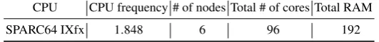
Table 1.Specifications of cluster system Oakleaf-FX to solve the134-dimension SVP Challenge; note that the units of “CPU frequency” and “Total RAM” areGHzandGB, respectively
CPU CPU frequency # of nodes Total # of cores Total RAM
SPARC64 IXfx 1.848 6 96 192
are the most costly parts of our algorithm, it is important to optimize the choices ofS
andS′; however, these sets differ only in their size. Note that NNRs in S andS′ are chosen by ascending order of expectation of squared lengths (shown in Theorem 2) of generated lattice vectors with several bases.
The purpose of the lattice vector generation with S (at line 5 in Algorithm 1) is finding relatively short lattice vectors, so the size ofSshould be large. The purpose of the other lattice vector generation withS′(at line 4 in Algorithm 2) is decreasing the sum of squared length of orthogonal basis vectors and generating many lattice bases variants as mentioned in Section 5.2 by repeatedly applying lattice reduction (e.g., the LLL algorithm), so it is not necessary to choose the size ofS′as large.
Actually, we adjust the parametersℓlc,δ,δ′,δ′′, and sizes of setsSandS′in such a way that the calculation times of two lattice vector generations withSandS′are around several minutes. More concretely, we chose the parameters such that the calculation times are5minutes and10minutes, respectively, and the lattice vector generation with
S′is repeatedly evaluated around500times per one Algorithm 2 evaluation on average when we found a solution of a150-dimensional problem instance of the SVP Challenge.
6
Application to SVP Challenge
The shortest vector problem (SVP) is an important problem because of its relation to the security strength of lattice-based cryptosystems, and studying algorithms for solving it is an important research topic. The SVP Challenge was started in 2010 [45] as a way of advancing this research. The challenge provides a problem instance generator and accepts submissions of discovered short lattice vectors. As mentioned in Section 2.3, a submitted lattice vector of a lattice L is inducted into the hall-of-fame if its length is less than1.05·GH(L)and less than the lengths of other registered lattice vectors if they exist for the same dimension.
6.1 Equipment
We applied our algorithm to the problems in the SVP Challenge. In this section, we explain our equipment and results.
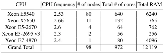
Table 2.Specifications of cluster system Chimera to solve SVP Challenge instances of138,140, 142,144,146,148, and150dimensions; note that the units of “CPU frequency” and “Total RAM” areGHzandGB, respectively
CPU CPU frequency # of nodes Total # of cores Total RAM
Xeon E5540 2.53 80 640 6240
Xeon X5650 2.66 11 132 765
Xeon E5-2670 2.6 4 64 762
Xeon E5-2695 v3 2.3 2 56 256
Xeon E7-4870 2.4 1 80 4096
Grand Total 98 972 12 119
Table 3.Specifications of cluster system ASGC to solve148and150-dimensions instances of SVP Challenge; note that the units of “CPU frequency” and “Total RAM” areGHzand GB, respectively
CPU CPU frequency # of nodes Total # of cores Total RAM
Xeon E5-2680 v2 2.8 5 100 640
Intel C++ Compiler version 14.0.2, Intel MPI Library version 4.1, and TORQUE sion 4.2.8 in the ASGC, and Intel C++ Compiler version 16.0.3, Intel MPI Library ver-sion 5.1, and PBS Profesver-sional 13.1 in the Reedbush-U. Note that Hyper-Threading was enabled and Turbo Boost was disabled in all nodes of Chimera, while Hyper-Threading was disabled and Turbo Boost was disabled in all nodes of ASGC and Reedbush-U. Note also that these clusters were shared systems, so all the processes were controlled by the job schedulers. Now, let us briefly explain the pre-processing. Before executing processes for our algorithm, the lattice basis of the input was pre-processed. We used the BKZ algorithm implemented by fplll [50] to reduce components of the lattice basis to small integers.
For each process when we solve the problem instances, the process-unique informa-tionpuiwas given as the rank by the MPI libraries and job schedulers, namely, thepui value ranged from0tom−1, wheremis the number of requested processes sent to the MPI libraries and job schedulers.
6.2 Experimental Results
We used our algorithm to solve SVP Challenge problem instances of 134,138,140, 142,144,146,148, and150dimensions with seed0. We used FX10 to solve the134 -dimensional instance, Chimera to solve the instances with 138–146 dimensions, and the two clusters Chimera and ASGC to solve the148-dimensional instance.
Table 4.Specifications of cluster system Reedbush-U to solve the150-dimensional instance of the SVP Challenge; note that the units of “CPU frequency” and “Total RAM” areGHzandGB, respectively
CPU CPU frequency # of nodes Total # of cores Total RAM
Xeon E5-2695 v4 2.1 24 864 5856
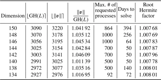
Table 5.Our experimental results for the SVP Challenge instances of dimensions134,138,140, 142,144,146,148, and150, where “GH(L)” is the Gaussian heuristic of a given latticeL, “v” in the column header indicates a solution of the corresponding row, the “Max. # of requested processes” column shows the maximum number of requested processes sent to the job schedulers, and the “Days to solve” column lists the wall-clock times to obtain each solution
Dimension ⌊GH(L)⌉ ⌊∥v∥⌉ ∥v∥ GH(L)
Max. # of requested processes
Days to solve
Root Hermite
factor
150 3090 3220 1.041 92 864 394 1.007 68 148 3070 3178 1.035 12 1000 256 1.007 69 146 3056 3195 1.045 34 1000 64 1.007 83 144 3025 3154 1.042 84 700 50 1.007 87 142 3003 3141 1.046 09 700 50 1.007 96 140 2991 3025 1.011 39 500 50 1.007 78 138 2972 3077 1.035 16 500 140 1.008 01 134 2927 2976 1.016 95 92 72 1.008 01
respectively. We did not use these computing nodes simultaneously. Therefore, the total wall-clock time was about 394 days. Note that when we used the computing node (1), we requested 24 processes for job schedulers and the other cases (2), (3), (4), and (5), and the number of requested processes was the same as the number of cores.
When we found a solution of the150-dimensional instance, tuned parameters of our algorithm were as follows:ℓfc =50,ℓlc =50,δ =0.9999,δ′=0.985,δ′′ =0.0002, δstock=1.08,ℓlink=50, andΘ=0.93. The method we used to choose these parameters is explained in Section 5.3.
We clarify the numbers of lattice vectors generated by the two subroutines in line 5 in Algorithm 1 with a setSof NNRs and in line 4 in Algorithm 2 with a setS′of NNRs, and the costs per generation when we solved the150-dimensional problem and problems with a smaller dimensions less than150. The sizes ofSandS′are around30millions NNRs and50thousands NNRs, respectively. Note that lines 3-19 in Algorithm 2 are repeated until the termination condition in line 18 is satisfied, and the number of loops is500on average. The calculation times of the lattice vector generations withSandS′
are around5minutes and10minutes, respectively. That is, the calculation time of these generations per lattice vector is around12-20micro-seconds.
104
105
106
107
108
109
1010
1011
1012
110 120 130 140 150 160
Single
thread
calculation
time
in
seconds
Dimension
Ourresults
Fittingbasedonourresults
OtherresultsinSVPChallenge
Fittingbasedonotherresults
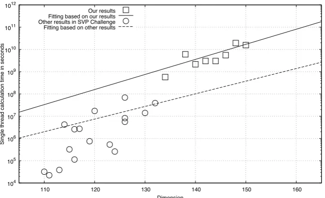
Fig. 1. Comparison of solved dimension and single thread calculation time in seconds of our results and results in the SVP Challenge, where plotted boxes are our8results, the straight solid line is fitted to our results, plotted circles are other17results of problems with dimensions greater than or equal to100and specified overall calculation times, and the dotted line is fitted to these results
the remaining stock vectors and link vectors is around60gigabytes. We estimate that the total size of all the found stock vectors and link vectors is several hundred gigabytes for solving the150-dimensional problem.
Table 5 lists the details of our solutions. The solution of the150-dimensional problem is the current world record.
We show a comparison of solved dimension and single thread calculation time in seconds of our results and the results from the SVP Challenge in Figure 1. In this figure, plotted boxes are our8results, and plotted circles are other17results for problems with dimensions greater than or equal to100and specified overall calculation times. It is clear that our algorithm outperforms others. This is experimental evidence that our proposal is effective at reducing higher-dimensional lattice bases and solving higher-dimensional SVPs.
Additionally, we show fittings of our and the SVP Challenge results in Figure 1 obtained byfitfunction of GNU Plot version5.2. As a result, we obtained the straight solid line for our results and the dotted line for the other SVP Challenges results. Note that these lines are expressed as f(x) =cax+b+d with four variablesa,b,c,d. Obtained values and asymptotic standard errors of a,b,c,d, and values of the root mean square (RMS) of residuals by using fitare as follows: a = 1.002 87±933.3,
b=0.988 369±5095,c=1.146 25±123.6, andd =1.0004±5.792×10⁷, and the value of RMS is1.666 35×107for the dotted line.
7
Conclusion
We proposed an algorithm suitable for parallel computing environments to reduce the lattice basis and presented its results in the SVP Challenge.
Regarding the results in the SVP Challenge, we discovered solutions to problem instances of dimensions134,138,140,142,144,146,148, and150, a world record for the highest dimension. This is clear experimental evidence that our proposal is effective at reducing the lattice basis and solving the SVP by using a parallel computing environment.
References
1. Agrawal, S., Boneh, D., Boyen, X.: Efficient lattice (H)IBE in the standard model. In: Gilbert [25], pp. 553–572,http://dx.doi.org/10.1007/978-3-642-13190-5_28
2. Agrawal, S., Freeman, D.M., Vaikuntanathan, V.: Functional encryption for inner product predicates from learning with errors. In: Lee and Wang [35], pp. 21–40,http://dx.doi. org/10.1007/978-3-642-25385-0_2
3. Ajtai, M.: The shortest vector problem inL2isNP-hard for randomized reductions (extended abstract). In: Vitter, J.S. (ed.) Proceedings of the Thirtieth Annual ACM Symposium on the Theory of Computing, Dallas, Texas, USA, May 23-26, 1998. pp. 10–19. ACM (1998),
http://doi.acm.org/10.1145/276698.276705
4. Ajtai, M., Dwork, C.: A public-key cryptosystem with worst-case/average-case equivalence. In: Leighton, F.T., Shor, P.W. (eds.) Proceedings of the Twenty-Ninth Annual ACM Sympo-sium on the Theory of Computing, El Paso, Texas, USA, May 4-6, 1997. pp. 284–293. ACM (1997),http://doi.acm.org/10.1145/258533.258604
5. Aono, Y., Nguyen, P.Q.: Random sampling revisited: Lattice enumeration with discrete pruning. In: Coron, J., Nielsen, J.B. (eds.) Advances in Cryptology - EUROCRYPT 2017 - 36th Annual International Conference on the Theory and Applications of Cryptographic Techniques, Paris, France, April 30 - May 4, 2017, Proceedings, Part II. Lecture Notes in Computer Science, vol. 10211, pp. 65–102 (2017), http://dx.doi.org/10.1007/ 978-3-319-56614-6_3
6. Aono, Y., Wang, Y., Hayashi, T., Takagi, T.: Improved progressive BKZ algorithms and their precise cost estimation by sharp simulator. In: Fischlin and Coron [19], pp. 789–819,
http://dx.doi.org/10.1007/978-3-662-49890-3_30
7. Boneh, D., Gentry, C., Gorbunov, S., Halevi, S., Nikolaenko, V., Segev, G., Vaikuntanathan, V., Vinayagamurthy, D.: Fully key-homomorphic encryption, arithmetic circuit ABE and compact garbled circuits. In: Nguyen, P.Q., Oswald, E. (eds.) Advances in Cryptology -EUROCRYPT 2014 - 33rd Annual International Conference on the Theory and Applications of Cryptographic Techniques, Copenhagen, Denmark, May 11-15, 2014. Proceedings. Lecture Notes in Computer Science, vol. 8441, pp. 533–556. Springer (2014),http://dx.doi.org/ 10.1007/978-3-642-55220-5_30
8. Brakerski, Z., Gentry, C., Vaikuntanathan, V.: (leveled) fully homomorphic encryption without bootstrapping. In: Goldwasser, S. (ed.) Innovations in Theoretical Computer Sci-ence 2012, Cambridge, MA, USA, January 8-10, 2012. pp. 309–325. ACM (2012),
9. Brakerski, Z., Gentry, C., Vaikuntanathan, V.: (leveled) fully homomorphic encryption without bootstrapping. TOCT 6(3), 13:1–13:36 (2014),http://doi.acm.org/10.1145/ 2633600
10. Brakerski, Z., Vaikuntanathan, V.: Efficient fully homomorphic encryption from (standard) LWE. In: Ostrovsky, R. (ed.) IEEE 52nd Annual Symposium on Foundations of Computer Science, FOCS 2011, Palm Springs, CA, USA, October 22-25, 2011. pp. 97–106. IEEE Computer Society (2011),http://dx.doi.org/10.1109/FOCS.2011.12
11. Brakerski, Z., Vaikuntanathan, V.: Efficient fully homomorphic encryption from (stan-dard) LWE. SIAM J. Comput. 43(2), 831–871 (2014),http://dx.doi.org/10.1137/ 120868669
12. Brakerski, Z., Vaikuntanathan, V.: Lattice-based FHE as secure as PKE. In: Naor, M. (ed.) Innovations in Theoretical Computer Science, ITCS’14, Princeton, NJ, USA, January 12-14, 2014. pp. 1–12. ACM (2014),http://doi.acm.org/10.1145/2554797.2554799
13. Buchmann, J., Ludwig, C.: Practical lattice basis sampling reduction. Cryptology ePrint Archive, Report 2005/072 (2005), https://eprint.iacr.org/2005/072, https:// eprint.iacr.org/2005/072
14. Buchmann, J.A., Ludwig, C.: Practical lattice basis sampling reduction. In: Hess, F., Pauli, S., Pohst, M.E. (eds.) Algorithmic Number Theory, 7th International Symposium, ANTS-VII, Berlin, Germany, July 23-28, 2006, Proceedings. Lecture Notes in Computer Science, vol. 4076, pp. 222–237. Springer (2006),http://dx.doi.org/10.1007/11792086_17
15. Chen, Y., Nguyen, P.Q.: BKZ 2.0: Better lattice security estimates. In: Lee and Wang [35], pp. 1–20,http://dx.doi.org/10.1007/978-3-642-25385-0_1
16. Dagdelen, Ö., Schneider, M.: Parallel enumeration of shortest lattice vectors. In: D’Ambra, P., Guarracino, M.R., Talia, D. (eds.) Euro-Par 2010 - Parallel Processing, 16th International Euro-Par Conference, Ischia, Italy, August 31 - September 3, 2010, Proceedings, Part II. Lecture Notes in Computer Science, vol. 6272, pp. 211–222. Springer (2010),http://dx. doi.org/10.1007/978-3-642-15291-7_21
17. Detrey, J., Hanrot, G., Pujol, X., Stehlé, D.: Accelerating lattice reduction with fpgas. In: Abdalla, M., Barreto, P.S.L.M. (eds.) Progress in Cryptology - LATINCRYPT 2010, First International Conference on Cryptology and Information Security in Latin America, Puebla, Mexico, August 8-11, 2010, Proceedings. Lecture Notes in Computer Science, vol. 6212, pp. 124–143. Springer (2010),http://dx.doi.org/10.1007/978-3-642-14712-8_8
18. Dwork, C. (ed.): Proceedings of the 40th Annual ACM Symposium on Theory of Computing, Victoria, British Columbia, Canada, May 17-20, 2008. ACM (2008)
19. Fischlin, M., Coron, J. (eds.): Advances in Cryptology - EUROCRYPT 2016 - 35th Annual International Conference on the Theory and Applications of Cryptographic Techniques, Vienna, Austria, May 8-12, 2016, Proceedings, Part I, Lecture Notes in Computer Science, vol. 9665. Springer (2016),http://dx.doi.org/10.1007/978-3-662-49890-3
20. Fukase, M., Kashiwabara, K.: An accelerated algorithm for solving SVP based on statistical analysis. JIP 23(1), 67–80 (2015),http://dx.doi.org/10.2197/ipsjjip.23.67
21. Gama, N., Nguyen, P.Q.: Finding short lattice vectors within mordell’s inequality. In: Dwork [18], pp. 207–216,http://doi.acm.org/10.1145/1374376.1374408
22. Gama, N., Nguyen, P.Q.: Predicting lattice reduction. In: Smart, N.P. (ed.) Advances in Cryptology - EUROCRYPT 2008, 27th Annual International Conference on the Theory and Applications of Cryptographic Techniques, Istanbul, Turkey, April 13-17, 2008. Proceedings. Lecture Notes in Computer Science, vol. 4965, pp. 31–51. Springer (2008),http://dx.doi. org/10.1007/978-3-540-78967-3_3
24. Gentry, C., Peikert, C., Vaikuntanathan, V.: Trapdoors for hard lattices and new cryptographic constructions. In: Dwork [18], pp. 197–206,http://doi.acm.org/10.1145/1374376. 1374407
25. Gilbert, H. (ed.): Advances in Cryptology - EUROCRYPT 2010, 29th Annual International Conference on the Theory and Applications of Cryptographic Techniques, French Riviera, May 30 - June 3, 2010. Proceedings, Lecture Notes in Computer Science, vol. 6110. Springer (2010),http://dx.doi.org/10.1007/978-3-642-13190-5
26. Goldreich, O., Goldwasser, S., Halevi, S.: Public-key cryptosystems from lattice reduction problems. In: Jr., B.S.K. (ed.) Advances in Cryptology - CRYPTO ’97, 17th Annual In-ternational Cryptology Conference, Santa Barbara, California, USA, August 17-21, 1997, Proceedings. Lecture Notes in Computer Science, vol. 1294, pp. 112–131. Springer (1997),
http://dx.doi.org/10.1007/BFb0052231
27. Gorbunov, S., Vaikuntanathan, V., Wee, H.: Attribute-based encryption for circuits. In: Boneh, D., Roughgarden, T., Feigenbaum, J. (eds.) Symposium on Theory of Computing Conference, STOC’13, Palo Alto, CA, USA, June 1-4, 2013. pp. 545–554. ACM (2013),http://doi. acm.org/10.1145/2488608.2488677
28. Gorbunov, S., Vaikuntanathan, V., Wee, H.: Attribute-based encryption for circuits. J. ACM 62(6), 45 (2015),http://doi.acm.org/10.1145/2824233
29. Gorbunov, S., Vaikuntanathan, V., Wee, H.: Predicate encryption for circuits from LWE. In: Gennaro, R., Robshaw, M. (eds.) Advances in Cryptology - CRYPTO 2015 - 35th Annual Cryptology Conference, Santa Barbara, CA, USA, August 16-20, 2015, Proceedings, Part II. Lecture Notes in Computer Science, vol. 9216, pp. 503–523. Springer (2015), http: //dx.doi.org/10.1007/978-3-662-48000-7_25
30. Hermans, J., Schneider, M., Buchmann, J.A., Vercauteren, F., Preneel, B.: Parallel shortest lattice vector enumeration on graphics cards. In: Bernstein, D.J., Lange, T. (eds.) Progress in Cryptology - AFRICACRYPT 2010, Third International Conference on Cryptology in Africa, Stellenbosch, South Africa, May 3-6, 2010. Proceedings. Lecture Notes in Com-puter Science, vol. 6055, pp. 52–68. Springer (2010), http://dx.doi.org/10.1007/ 978-3-642-12678-9_4
31. Hoffstein, J., Pipher, J., Silverman, J.H.: NTRU: A ring-based public key cryptosystem. In: Buhler, J. (ed.) Algorithmic Number Theory, Third International Symposium, ANTS-III, Portland, Oregon, USA, June 21-25, 1998, Proceedings. Lecture Notes in Computer Science, vol. 1423, pp. 267–288. Springer (1998),http://dx.doi.org/10.1007/BFb0054868
32. Hoffstein, J., Pipher, J., Silverman, J.H.: An Introduction to Mathematical Cryptography. Undergraduate Texts in Mathematics, Springer-Verlag, 1st edn. (2008),http://dx.doi. org/10.1007/978-0-387-77993-5
33. Kannan, R.: Improved algorithms for integer programming and related lattice problems. In: Johnson, D.S., Fagin, R., Fredman, M.L., Harel, D., Karp, R.M., Lynch, N.A., Papadimitriou, C.H., Rivest, R.L., Ruzzo, W.L., Seiferas, J.I. (eds.) Proceedings of the 15th Annual ACM Symposium on Theory of Computing, 25-27 April, 1983, Boston, Massachusetts, USA. pp. 193–206. ACM (1983),http://doi.acm.org/10.1145/800061.808749
34. Kuo, P., Schneider, M., Dagdelen, Ö., Reichelt, J., Buchmann, J.A., Cheng, C., Yang, B.: Extreme enumeration on GPU and in clouds - - how many dollars you need to break SVP challenges -. In: Preneel and Takagi [43], pp. 176–191,http://dx.doi.org/10.1007/ 978-3-642-23951-9_12
36. Lenstra, A.K., Lenstra, H.W., Lovász, L.: Factoring polynomials with rational coeffi-cients. Mathematische Annalen 261(4), 515–534 (1982),http://dx.doi.org/10.1007/ BF01457454
37. Ludwig, C.: Practical Lattice Basis Sampling Reduction. Ph.D. thesis, Technische Universität Darmstadt Universitäts (2005),http://elib.tu-darmstadt.de/diss/000640
38. Micciancio, D., Walter, M.: Fast lattice point enumeration with minimal overhead. In: Indyk, P. (ed.) Proceedings of the Twenty-Sixth Annual ACM-SIAM Symposium on Discrete Algo-rithms, SODA 2015, San Diego, CA, USA, January 4-6, 2015. pp. 276–294. SIAM (2015),
http://dx.doi.org/10.1137/1.9781611973730.21
39. Micciancio, D., Walter, M.: Practical, predictable lattice basis reduction. In: Fischlin and Coron [19], pp. 820–849,http://dx.doi.org/10.1007/978-3-662-49890-3_31
40. Nguyen, P.Q., Vallée, B. (eds.): The LLL Algorithm - Survey and Applications. In-formation Security and Cryptography, Springer (2010),http://dx.doi.org/10.1007/ 978-3-642-02295-1
41. Pieterse, V., Black, P.E.: “single program multiple data” in Dictionary of Algorithms and Data Structures (December 2004),http://www.nist.gov/dads/HTML/singleprogrm.html
42. Plantard, T., Schneider, M.: Creating a challenge for ideal lattices. Cryptology ePrint Archive, Report 2013/039 (2013),https://eprint.iacr.org/2013/039
43. Preneel, B., Takagi, T. (eds.): Cryptographic Hardware and Embedded Systems - CHES 2011 - 13th International Workshop, Nara, Japan, September 28 - October 1, 2011. Proceedings, Lecture Notes in Computer Science, vol. 6917. Springer (2011)
44. Regev, O.: On lattices, learning with errors, random linear codes, and cryptography. In: Gabow, H.N., Fagin, R. (eds.) Proceedings of the 37th Annual ACM Symposium on Theory of Computing, Baltimore, MD, USA, May 22-24, 2005. pp. 84–93. ACM (2005), http: //doi.acm.org/10.1145/1060590.1060603
45. Schneider, M., Gama, N.: SVP Challenge, http://www.latticechallenge.org/ svp-challenge/
46. Schneider, M., Göttert, N.: Random sampling for short lattice vectors on graph-ics cards. In: Preneel and Takagi [43], pp. 160–175, http://dx.doi.org/10.1007/ 978-3-642-23951-9_11
47. Schnorr, C.: Lattice reduction by random sampling and birthday methods. In: Alt, H., Habib, M. (eds.) STACS 2003, 20th Annual Symposium on Theoretical Aspects of Computer Sci-ence, Berlin, Germany, February 27 - March 1, 2003, Proceedings. Lecture Notes in Com-puter Science, vol. 2607, pp. 145–156. Springer (2003),http://dx.doi.org/10.1007/ 3-540-36494-3_14
48. Schnorr, C.: Correction to lattice reduction by random sampling and birthday methods.http:
//www.math.uni-frankfurt.de/~dmst/research/papers.html(February 2012)
49. Schnorr, C., Euchner, M.: Lattice basis reduction: Improved practical algorithms and solving subset sum problems. Math. Program. 66, 181–199 (1994),http://dx.doi.org/10.1007/ BF01581144